In previous section we discussed about Data Handling in R
Huge amount of data stored on the servers can be accessed through SQL(Structured Query Language). R is compatible with these databases. For SQL server, this is done through ODBC. However, few steps needs to be followed to link R to the database. All you need to do is
- Create ODBC from the SQL Server
- To create ODBC, the following link https://www.youtube.com/watch?v=2xQX76nEdvo can be followed.
Once ODBC is created, we need to connect ODBC with R. For the connection, we need to install a package called RODBC in R. Once the package is installed, it is loaded into the current workspace, by calling the function, library(RODBC). This will load the functions available in the RODBC package into the current workspace for further use. The following syntax shows, how to load the package, and further connect R with Database.
> library(RODBC)
> conn <- odbcConnect(“dblink", uid=“uid", pwd=“passwd")
> salesdata <- sqlFetch(conn, “sales")
> ordersdat <- sqlQuery(conn, "select * from orders")
> close(conn)
> dbhandle <- odbcDriverConnect('driver={SQL Server}; server=MyServerName;   database = MyDbName; trusted_connection=true')
In the above-mentioned commands, “MyServerName” & “MyDbName” is replaced with our server and database names. We should make sure that we have access to that server and database before connecting. Once the data is imported, the connection is closed using the function close().
spend_row_count<-sqlQuery(dbhandle, “select count(*) from MyTable”)
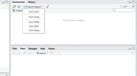
Importing dataset using GUI
An easy to use Graphical User Interface can be used to import the data from different formats into R. Steps to be followed are shown below.

Working with Datasets
Once the dataset is imported/connected, there are some basic validation checks that we have to make, before going for further analysis.
- Is the data imported correctly?
- Are the variables imported in right format?
- Did we import all the rows and columns?
Data preparation is an important step in the field of data analysis. Importing, exploring, validating and sanitizing the data are as important as data analysis. It is always a good practice to do some basic checks to get an idea on the dataset. We have a look on the number of rows, columns, the variable structures, data snapshot summary, etc. It is important to check if there are any missing values, or if there are any outliers lying in the data set. For example: If the age is recorded as 1200, then there has been a problem in recording or importing the data. Hence fixing the imported data is equally important. One can validate the dataset by verifying its structure. By structure, we mean the number of rows and columns, the format of data, the limits of the values taken by the data columns, etc. We can also have a look at the summary of the data.
There are three important rules in the field of data handling – Importing, Rectifying, and Applying.
Import: The data stored in different formats can be imported in R, by using basic commands like read.csv() for csv files, read.xlsx() for xlsx files and other commands for different formats.
Rectify: After the data is imported into R, it is important to check the accuracy of the data i.e. the degree of correctness of data. It is important to check if there is any data missing, or if there is an outlier lying in the data set. Taking an example: if the age is recorded as 12 and the education is recorded as Graduation, then there has been a problem in recording the survey data. Hence fixing the imported data is equally important.
Let’s see some commands to perform some basic checks on the dataset without actually opening it.
Basic Commands on the Datasets
dim()
This function returns the number of rows and columns. From this we can have a quick idea on the data import. If we don’t have the number of rows and columns as expected, we can address the issue at that phase itself.
> dim(Sales)
## [1] 11 7
The output says that that the data set Sales has 11 rows and 7 columns
names()
This function can be used to get or set the names of the variables in the dataset. Sometimes import doesn’t consider column names while importing from text files, so we need to be careful while importing.
>names(Sales)
## [1] “custId” “custName” “custCountry” “productSold”
## [5] “salesChannel” “unitsSold” “dateSold”
In this output we can see the names of the 7 columns in the data set Sales.
head()
head() returns the first 6 observations of the data set. This function is used to have a quick look at the first few records of the data. head() can be used to limit the number of observations in the output.
>head(Sales)
##   custId     custName                  custCountry productSold
## 1  23262 Candice Levy                        Congo     SUPA101
## 2  23263 Xerxes Smith                       Panama     DETA200
## 3  23264 Levi Douglas Tanzania, United Republic of     DETA800
## 4  23265 Uriel Benton                 South Africa     SUPA104
## 5  23266 Celeste Pugh                        Gabon     PURA200
## 6  23267 Vance Campos         Syrian Arab Republic     PURA100
##   salesChannel unitsSold  dateSold
## 1       Retail       117  8/9/2012
## 2       Online        73  7/6/2012
## 3       Online       205 8/18/2012
## 4       Online        14  8/5/2012
## 5       Retail       170 8/11/2012
## 6       Retail       129 7/11/2012
The output above displays the first 6 observations of Sales
tail()
tail() returns the last 6 observations of the data set. This function is used as a substitute to the function, head() wherever it is applicable
> tail(Sales)
##    custId           custName              custCountry productSold
## 6   23267       Vance Campos     Syrian Arab Republic     PURA100
## 7   23268       Latifah Wall               Guadeloupe     DETA100
## 8   23269     Jane Hernandez                Macedonia     PURA100
## 9   23270        Wanda Garza               Kyrgyzstan     SUPA103
## 10  23271 Athena Fitzpatrick                  Reunion     SUPA103
## 11  23272      Anjolie Hicks Turks and Caicos Islands     DETA200
##    salesChannel unitsSold  dateSold
## 6        Retail       129 7/11/2012
## 7        Retail        82 7/12/2012
## 8        Retail       116  6/3/2012
## 9        Online        67  6/7/2012
## 10       Retail       125 7/27/2012
## 11       Retail        71 7/31/2012
The output above shows the last 6 observations of Sales
str()
str() is an important function which returns the complete structure of the data set. This would include the number of rows and columns, the names of the columns, the type or class of data set contained in these columns, and it even gives a brief summary on the information contained in these columns.
> str(Sales)
## 'data.frame':    11 obs. of  7 variables:
##  $ custId      : int  23262 23263 23264 23265 23266 23267 23268 23269 23270 23271 ...
##  $ custName    : Factor w/ 11 levels "Anjolie Hicks",..: 3 11 7 8 4 9 6 5 10 2 ...
##  $ custCountry : Factor w/ 11 levels "Congo","Gabon",..: 1 6 10 8 2 9 3 5 4 7 ...
##  $ productSold : Factor w/ 8 levels "DETA100","DETA200",..: 6 2 3 8 5 4 1 4 7 7 ...
##  $ salesChannel: Factor w/ 2 levels "Online","Retail": 2 1 1 1 2 2 2 2 1 2 ...
##  $ unitsSold   : int  117 73 205 14 170 129 82 116 67 125 ...
##  $ dateSold    : Factor w/ 11 levels "6/3/2012","6/7/2012",..: 11 7 9 10 8 3 4 1 2 5 ...
We can use this function to see the detailed summary of a single variable. $ can be used to mention the particular column name for which the data is to be verified.
> str(Sales$unitsSold)
## int [1:11] 117 73 205 14 170 129 82 116 67 125 ...
Print()
Print() can be used to display the data set on the console itself. It works well if the data set is small.
> print(Sales)
##    custId           custName                  custCountry productSold
## 1   23262       Candice Levy                        Congo     SUPA101
## 2   23263       Xerxes Smith                       Panama     DETA200
## 3   23264       Levi Douglas Tanzania, United Republic of     DETA800
## 4   23265       Uriel Benton                 South Africa     SUPA104
## 5   23266       Celeste Pugh                        Gabon     PURA200
## 6   23267       Vance Campos         Syrian Arab Republic     PURA100
## 7   23268       Latifah Wall                   Guadeloupe     DETA100
## 8   23269     Jane Hernandez                    Macedonia     PURA100
## 9   23270        Wanda Garza                   Kyrgyzstan     SUPA103
## 10  23271 Athena Fitzpatrick                      Reunion     SUPA103
## 11  23272      Anjolie Hicks     Turks and Caicos Islands     DETA200
##    salesChannel unitsSold  dateSold
## 1        Retail       117  8/9/2012
## 2        Online        73  7/6/2012
## 3        Online       205 8/18/2012
## 4        Online        14  8/5/2012
## 5        Retail       170 8/11/2012
## 6        Retail       129 7/11/2012
## 7        Retail        82 7/12/2012
## 8        Retail       116  6/3/2012
## 9        Online        67  6/7/2012
## 10       Retail       125 7/27/2012
## 11       Retail        71 7/31/2012
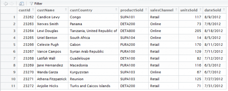
View()
The View() function gives a better-formatted snapshot of the dataset. Print function prints the dataset in the console. If there are many columns in the dataset, then we may not be able to get a good view of the dataset.
>View(Sales)

| Code | Description |
|---|---|
| dim(Sales) | To check the number of rows and columns |
| names(Sales) | What are the column names?, Sometimes import doesn’t consider column names while |
| importing | |
| head(Sales) | First few observations of data |
| tail(Sales) | Last few observations of the data |
| str(Sales) | Structure of the whole data, are all the variables in the expected format |
| str(Sales$unitsSold) | Structure of few important variables |
| View(Sales) | A snapshot of small datasets |
| Print(Sales) | Print the data if it is small |
Other useful commands
Few more examples are stated in the table below. Give them a try and find if the output matches with the description.
| Code | Description |
|---|---|
| str(Sales) | Get an idea on numeric and non numeric variables |
| summary(Sales) | Overall data summary |
| summary(Sales$unitsSold) | Get summary on numerical variables |
| table(Sales$unitsSold) | Get frequency tables for categorical variables |
| table(Sales$custCountry) | Get frequency tables for categorical variables |
| sum(is.na(Sales)) | Missing value count in full data |
| sum(is.na(Sales$unitsSold)) | Missing value count in a variable |
In the next post we will see Sub Setting in R.


