Before start our lesson please download the datasets.
Support Vector Machines
Statinfer.com
Contents
- Introduction
- The decision boundary with largest margin
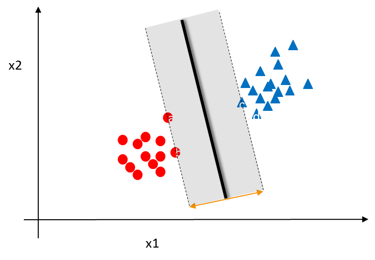
- SVM- The large margin classifier
- SVM algorithm
- The kernel trick
- Building SVM model
- Conclusion
Introduction
SVM is one more black box method in Machine Learning.Compared to other Machine Learning algorithms, SVM is totally a different approach to learning.SVM was first introduced by Vapnik and Chervonenkis and initially it was majorly compared with Neural Networks.Neural Networks has some issue with overfitting and computation time.The real theory behind SVM is not very straightward to understand but with some effort let us try to understand. The in-depth theory and mathematics of SVM needs great knowledge in vector algebra and numerical analysis .We will try to learn the basic principal, philosophy, implementation of SVM.SVM algorithm has better generalization ability. There are many applications where SVM works better than neural networks. Most of the times SVM takes lesser computation time than Neural Networks.To understand the SVM algorithm we will start with the Classifier.
Classifier
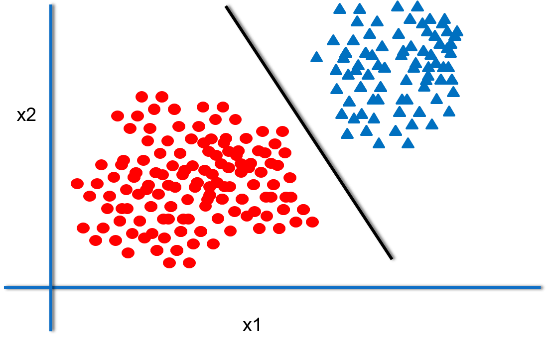
Classifier is nothing but a line that separates two classes. A good classifier is the one that generalizes well and work well on both training and testing data. Classifier need not be a straight line always. Classifiers need not be uniqe they can be many classifiers that does a good job of separating good from bad. From these multipe classifiers how do we will choose the best classifier. Solution for this is the “Margin of Classifier”
Margin of Classifier
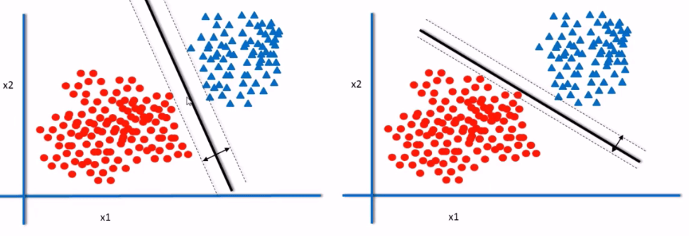
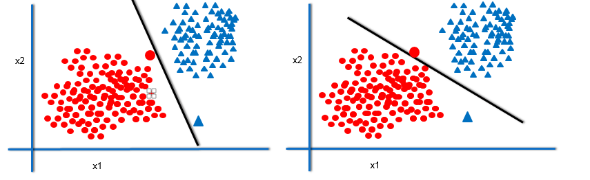
From the above picture we observed that there are two classifiers. If you see the margin from the classifier to the nearest data points it shows that classifier1 has the largest margin when compared to classifier2. The classifier that has the maximum margin will generalize well.But why?
Let us see this through an example
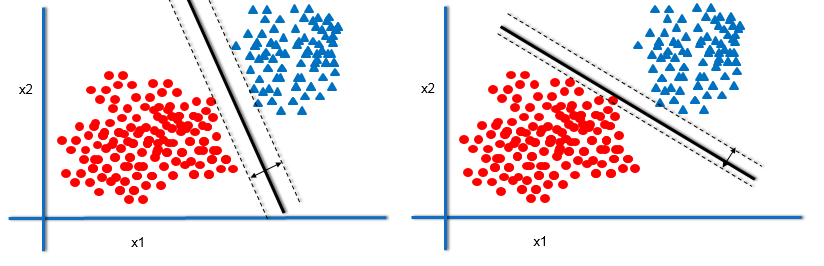
From the above picture we observed that there are two new data points there are at pretty much at the same location in the two graphs.Classifier1 still holds good it is still doing good job in separating the blue and red data points whereas classifier2 failed in both cases here blue triangle is classified as “RED” and Red circular point is classified as “BLUE” because it is working well on training data but when we take testing data on new data points classifier1 with maximum margin works better compared to classifier2 with smaller margin .SO, the decision boundary or classifier with the maximum Margin is the best Classifier.
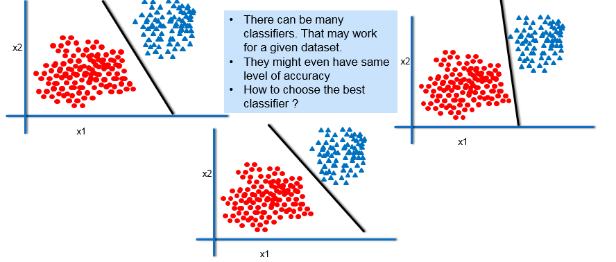
Many Classifiers
The Margin of Classifier
Out of all the classifiers, the one that has maximum margin will generalize well. But why?
The Best Decision Boundary
- Imagine two more data points. The classifier with maximum margin will be able to classify them more accurately.
The Maximum Margin Classifier
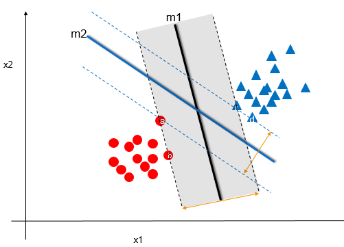
From the above picture we observed that there are two classifiers:m1 and m2. m1 has larger margin and m1 is close to data points a,b and c whereas m2 is having lesser margin when compared with m1 and it is close to data points a,c and d.So, the best classifier out of this two will be m1 because it has large margin. For a given dataset the classifier that has maximum margin will have maximum training accuracy and testing accuracy.So, we would generally prefer the classifier that has maximum margin.
## LAB: Simple Classifiers
- Dataset: Fraud Transaction/Transactions_sample.csv
- Draw a classification graph that shows all the classes
- Build a logistic regression classifier
- Draw the classifier on the data plot

## Solution
#Importing the dataset:
import pandas as pd
Transactions_sample = pd.read_csv("datasets/Fraud Transaction/Transactions_sample.csv")
Transactions_sample.head(6)
#Name of the columns
Transactions_sample.columns
#The clasification graph distinguishing the two classes with colors or shapes.
import matplotlib.pyplot as plt
%matplotlib inline
fig = plt.figure()
ax1 = fig.add_subplot(111)

ax1.scatter(Transactions_sample.Total_Amount[Transactions_sample.Fraud_id==0],Transactions_sample.Tr_Count_week[Transactions_sample.Fraud_id==0], s=10, c='b', marker="o", label='Fraud_id=0')
ax1.scatter(Transactions_sample.Total_Amount[Transactions_sample.Fraud_id==1],Transactions_sample.Tr_Count_week[Transactions_sample.Fraud_id==1], s=10, c='r', marker="+", label='Fraud_id=1')
plt.legend(loc='upper left');
plt.show()

#build a logistic regression model
###Logistic Regerssion model1
import statsmodels.formula.api as sm
model1 = sm.logit(formula='Fraud_id ~ Total_Amount+Tr_Count_week', data=Transactions_sample)
fitted1 = model1.fit()
fitted1.summary()
# Getting slope and intercept of the line
#coefficients
coef=fitted1.normalized_cov_params
print(coef)

slope1=coef.Intercept[1]/(-coef.Intercept[2])
intercept1=coef.Intercept[0]/(-coef.Intercept[2])
import matplotlib.pyplot as plt

fig = plt.figure()
ax1 = fig.add_subplot(111)

ax1.scatter(Transactions_sample.Total_Amount[Transactions_sample.Fraud_id==0],Transactions_sample.Tr_Count_week[Transactions_sample.Fraud_id==0], s=30, c='b', marker="o", label='Fraud_id 0')
ax1.scatter(Transactions_sample.Total_Amount[Transactions_sample.Fraud_id==1],Transactions_sample.Tr_Count_week[Transactions_sample.Fraud_id==1], s=30, c='r', marker="+", label='Fraud_id 1')

plt.xlim(min(Transactions_sample.Total_Amount), max(Transactions_sample.Total_Amount))
plt.ylim(min(Transactions_sample.Tr_Count_week), max(Transactions_sample.Tr_Count_week))

plt.legend(loc='upper left');

x_min, x_max = ax1.get_xlim()
ax1.plot([0, x_max], [intercept1, x_max*slope1+intercept1])
plt.show()

#Accuracy of the model
#Creating the confusion matrix
predicted_values=fitted1.predict(Transactions_sample[["Total_Amount"]+["Tr_Count_week"]])
print('Predicted Values: ', predicted_values[1:10])

threshold=0.5

import numpy as np
predicted_class=np.zeros(predicted_values.shape)
predicted_class[predicted_values>threshold]=1

print('Predicted Class: ', predicted_class)

from sklearn.metrics import confusion_matrix as cm
ConfusionMatrix = cm(Transactions_sample[['Fraud_id']],predicted_class)
print('Confusion Matrix: ', ConfusionMatrix)

accuracy=(ConfusionMatrix[0,0]+ConfusionMatrix[1,1])/sum(sum(ConfusionMatrix))
print('Accuracy: ', accuracy)

error=1-accuracy
print('Error: ', error)
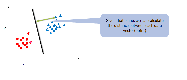
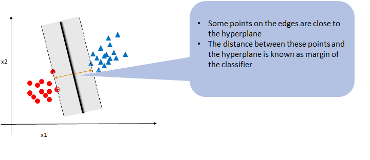
SVM- The large margin classifier
SVM is all about the finding the maximum-margin Classifier. Classifier is a generic name, mathematically it is called as hyper plane. Imagine in a 2Dimensional plane it is a kind of line.SVM uses the nearest training data points in the objective space. Based on them SVM finds the hyperplane or classifier. Each data point is considered as a p-dimensional vector(a list of p numbers).To find the optimal hyperplane that has maximum margin SVM uses vector algebra and mathematical optimization.
The SVM Algorithm

- If a dataset is linearly separable then we can always find a hyperplane f(x) such that
- For all negative labeled records f(x)<0
- For all positive labeled records f(x)>0
- This hyper plane f(x) is nothing but the linear classifier
- $f(x)=w_1 x_1+ w_2 x_2 +b$
- $f(x)=w^T x+b$

Math behind SVM Algorithm
SVM Algorithm – The Math
If you already understood the SVM technique and If you find this slide is too technical, you may want to skip it. The tool will take care of this optimization
- $f(x)=w^T x+b$
- $(w^T x^+ +b=1$ and $w^T x^- +b = -1$
- $x^+ = x^- + \lambda w$
- $w^T x^+ +b=1$
- $w^T(x^- + \lambda w)+b=1$
- $w^T x^- +\lambda w.w+b=1$
- $-1+\lambda w.w=1$
- $\lambda = 2/w.w$
- $m =|x^+ – x^-|$
- $m=|\lambda w|$
- $m=(2/w.w)*|w|$
- $m=2/||w||$
- Objective is to maximize $2/||w||$
- i.e minimize $||w||$
- A good decision boundary should be
- $w^T x^+ +b>=1$ for all y=1
- $w^T x^- +b<=-1$ for all y=-1
- i.e $ y(w^T x+b)>=1$ for all points
- Now we have the optimization problem with objective and constraints
- minimize $||w||$ or $(½)*||w||^2$
- With constant $y(w^T x+b)>=1$
- We can solve the above optimization problem to obtain w & b
SVM Result
SVM is all about fitting the Hyperplane that has maximum margin.SVM output doesnt contain any probability.It directly gives which class the new data point belongs to. For a new point xk calculate w^T x_k +b. If this value is positive then the prediction is positive else negative.At the end of SVM as a result we get the class of that particular new data point we will not get any probability as a result.
SVM on Python
- There are multiple SVM libraries available in Python.
- The package ‘Scikit’ is the most widely used for machine learning.
- There is a function called svm() within ‘Scikit’ package.
- There are various options within svm() function to customize the training process.
LAB: First SVM Learning Problem
- Dataset: Fraud Transaction/Transactions_sample.csv
- Draw a classification graph that shows all the classes
- Build a SVM classifier
- Draw the classifier on the data plots
- Predict the (Fraud vs not-Fraud) class for the data points Total_Amount=11000, Tr_Count_week=15 & Total_Amount=2000, Tr_Count_week=4
- Download the complete Dataset: Fraud Transaction/Transaction.csv
- Draw a classification graph that shows all the classes
- Build a SVM classifier
- Draw the classifier on the data plots
# Importing the sample data
import pandas as pd
Transactions_sample= pd.read_csv("datasets\\Fraud Transaction\\Transactions_sample.csv")
X = Transactions_sample[['Total_Amount']+['Tr_Count_week']]  # we only take the first two features. We could
                      # avoid this ugly slicing by using a two-dim dataset
y = Transactions_sample[['Fraud_id']].values.ravel()
#Drawing a classification graph of all classes
import matplotlib.pyplot as plt

plt.scatter(X['Total_Amount'], X['Tr_Count_week'], c=y, cmap=plt.cm.Paired)
plt.show()

#Building a SVM Classifier in python
from sklearn import svm
import numpy
X = Transactions_sample[['Total_Amount']+['Tr_Count_week']]  # we only take the first two features. We could
                      # avoid this ugly slicing by using a two-dim dataset
y = Transactions_sample[['Fraud_id']].values.ravel()

clf = svm.SVC(kernel='linear')
model =clf.fit(X,y)

Predicted = numpy.zeros(50)

# NOTE: If i is in range(0,n), then i takes vales [0,n-1]
for i in range(0,50):
    a = Transactions_sample.Total_Amount[i]
    b = Transactions_sample.Tr_Count_week[i]
    Predicted[i]=clf.predict([[a,b]])
    del a,b
#Plotting in SVM
import matplotlib.pyplot as plt
plt.scatter(X['Total_Amount'], X['Tr_Count_week'], c=y, cmap=plt.cm.Paired)
w = clf.coef_[0]
o = -w[0] / w[1]
plt.xlim(min(Transactions_sample.Total_Amount), max(Transactions_sample.Total_Amount))
x_min, x_max = ax1.get_xlim()
xx = np.linspace(x_min, x_max)
yy = o * xx - (clf.intercept_[0]) / w[1]

plt.plot(xx, yy, 'k-')
plt.show()

#Predict the (Fraud vs not-Fraud) class for the data points Total_Amount=11000, Tr_Count_week=15 & Total_Amount=2000, Tr_Count_week=4
#Prediction in SVM
new_data1=[11000, 15]
new_data2=[2000,4]

#Predict the (Fraud vs not-Fraud) class for the data points Total_Amount=11000, Tr_Count_week=15 & Total_Amount=2000, Tr_Count_week=4
NewPredicted1=model.predict([new_data1])
print(NewPredicted1)

NewPredicted2=clf.predict([new_data2])
print(NewPredicted2)
# Importing the whole dataset
import pandas as pd
Transactions= pd.read_csv("datasets\\Fraud Transaction\\Transaction.csv")
X = Transactions[['Total_Amount']+['Tr_Count_week']]  # we only take the first two features. We could
                      # avoid this ugly slicing by using a two-dim dataset
y = Transactions[['Fraud_id']].values.ravel()
#Drawing a classification graph of all classes
import matplotlib.pyplot as plt

plt.scatter(X['Total_Amount'], X['Tr_Count_week'], c=y, cmap=plt.cm.Paired)
plt.show()

#Build a SVM classifier
clf = svm.SVC(kernel='linear')
Smodel =clf.fit(X,y)
#Plotting in SVM
import matplotlib.pyplot as plt
plt.scatter(X['Total_Amount'], X['Tr_Count_week'], c=y, cmap=plt.cm.Paired)
w = clf.coef_[0]
o = -w[0] / w[1]
plt.xlim(min(Transactions_sample.Total_Amount), max(Transactions_sample.Total_Amount))
x_min, x_max = ax1.get_xlim()
xx = np.linspace(x_min, x_max)
yy = o * xx - (clf.intercept_[0]) / w[1]
plt.plot(xx, yy, 'k-')
plt.show()

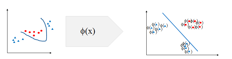
The Non-Linear Decision Boundary
Till now we have seen a linear classifier.what happens if the decision boundary is non-linear

From the above pictures we observed that there are positive classes then negative classes again some positive classes.In that case just fitting one line and finding the maximum margin wont be meaningful(since the decision boundary is not linear).when the decision boundary is non-linear SVM struggles to classify the classes.Infact SVM has no direct theory to set the non-linear decision boundary models.
To fit a non-linear boundary classifier we might have to create new variables or new dimensions in the data and see whether the decision boundary is linear. This phenomenon is called kernel trick..
what we do in kernel trick?
In kernel tree we try to increase the number of dimensions and try to make non-linear data into linear in a higher dimensional space
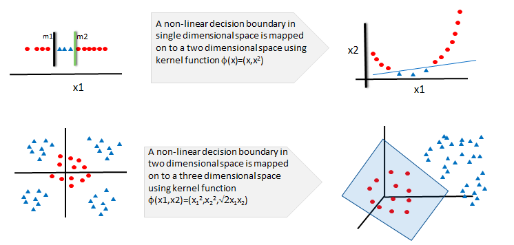
Mapping to Higher Dimensional Space
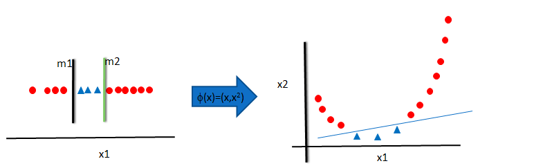
In this example we have 0’s then 1’s again 0’s this cant be directly linearly classifible.so what we try to do is we create a new variable called x2 it is just (x1)^2.so instead of just taking x1 one variable we will now use two variables x1 and x2 so we increase the dimension of this dataset by adding new variable. After adding new variable we can see our objective space is transformed into new dimensional space and we can clearly see a single linear decision boundary.
A single linear decision boundary is not possible in lower dimensional space we can increase the number of dimensions and then see whether we can fit a linear decision boundary. so, SVM doesnt have direct theory for non-linear decision boundary but we can increase the dimensions and we can use kernel trick to fit non-linear decision boundary.
Kernel Trick
Kernel Trick is the most important and trickiest part of SVM because most of the problems we see are not linearly separable. so when there is non-linear scenario then we have to use kernel Trick.
We used a function $\phi(x)=(x,(x^2))$ to transform the data x into a higher dimensional space. In the higher dimensional space, we could easily fit a liner decision boundary.This function $\phi(x)$ is known as kernel function and this process is known as kernel trick in SVM
Kernel trick solves the non-linear decision boundary problem much like the hidden layers in neural networks.Kernel trick is simply increasing the number of dimensions. It is to make the non-linear decision boundary in lower dimensional space as a linear decision boundary, in higher dimensional space. In simple words, Kernel trick makes the non-linear decision boundary to linear (in higher dimensional space)
Kernel Function Examples
| Name | Function | Type problem | ||||
|---|---|---|---|---|---|---|
| Polynomial Kernel | $(x_i^t x_j +1)^q$ q is degree of polynomial | Best for Image processing | ||||
| Sigmoid Kernel | $\tanh(ax_i^t x_j +k)$ k is offset value | Very similar to neural network | ||||
| Gaussian Kernel | $e^( | x_i – x_j | ^2/2 \sigma^2)$ | No prior knowledge on data | ||
| Linear Kernel | $1+x_i x_j min(x_i , x_j) – \frac{(x_i + x_j)}{2} min(x_i , x_j)^2 + \frac{min(x_i , x_j)^3}{3}$ | Text Classification | ||||
| Laplace Radial Basis Function (RBF) | $e^(-\lambda | x_i – x_j | ) , \lambda >= 0$ | No prior knowledge on data |
- There are many more kernel functions.
Choosing the Kernel Function
Choosing the kernel function is the most tricky part of the SVM and there is no specific theory that tells us that you should use this kernel function only.There is no proven theory that tells us which kernel function is going to work but there is lot of research going on that. In practice a low degree polynomial kernel or RBF kernel are generally used as trails.Choosing Kernel function is similar to choosing number of hidden layers in neural networks. Both of them have no proven theory to arrive at a standard value.As a first step, we can choose low degree polynomial or radial basis function or one of those from the list.
LAB: Kernel – Non linear classifier
- Dataset : Software users/sw_user_profile.csv
- How many variables are there in software user profile data?
- Plot the active users against and check weather the relation between age and “Active” status is linear or non-linear
- Build an SVM model(model-1), make sure that there is no kernel or the kernel is linear
- For model-1, create the confusion matrix and find out the accuracy
- Create a new variable. By using the polynomial kernel
- Build an SVM model(model-2), with the new data mapped on to higher dimensions. Keep the default kernel as linear
- For model-2, create the confusion matrix and find out the accuracy
- Plot the SVM with results.
- With the original data re-cerate the model(model-3) and let python choose the default kernel function.
- What is the accuracy of model-3?
#Dataset : Software users/sw_user_profile.csv
sw_user_profile = pd.read_csv("datasets/Software users/sw_user_profile.csv")
#How many variables are there in software user profile data?
sw_user_profile.shape
#Plot the active users against and check weather the relation between age and "Active" status is linear or non-linear
plt.scatter(sw_user_profile.Age,sw_user_profile.Id,color='blue')

#Build an SVM model(model-1), make sure that there is no kernel or the kernel is linear

#Model Building
X= sw_user_profile[['Age']]
y= sw_user_profile[['Active']].values.ravel()
Linsvc = svm.SVC(kernel='linear', C=1).fit(X, y)
#Predicting values
predict3 = Linsvc.predict(X)
#For model-1, create the confusion matrix and find out the accuracy
#Confusion Matrix
from sklearn.metrics import confusion_matrix
conf_mat = confusion_matrix(sw_user_profile[['Active']],predict3)
conf_mat
#Accuracy
Accuracy3 = Linsvc.score(X, y)
Accuracy3
New variable derivation. Mapping to higher dimensions
#Standardizing the data to visualize the results clearly
sw_user_profile['age_nor']=(sw_user_profile.Age-numpy.mean(sw_user_profile.Age))/numpy.std(sw_user_profile.Age)
#Create a new variable. By using the polynomial kernel
#Creating the new variable
sw_user_profile['new']=(sw_user_profile.age_nor)*(sw_user_profile.age_nor)
#Build an SVM model(model-2), with the new data mapped on to higher dimensions. Keep the default kernel as linear

#Model Building with new variable
X= sw_user_profile[['Age']+['new']]
y= sw_user_profile[['Active']].values.ravel()
Linsvc = svm.SVC(kernel='linear', C=1).fit(X, y)
predict4 = Linsvc.predict(X)
#For model-2, create the confusion matrix and find out the accuracy
#Confusion Matrix
conf_mat = confusion_matrix(sw_user_profile[['Active']],predict4)
conf_mat
#Accuracy
Accuracy4 = Linsvc.score(X, y)
Accuracy4
#With the original data re-cerate the model(model-3) and let python choose the default kernel function.
########Model Building with radial kernel function
X= sw_user_profile[['Age']]
y= sw_user_profile[['Active']].values.ravel()
Linsvc = svm.SVC(kernel='rbf', C=1).fit(X, y)
predict5 = Linsvc.predict(X)
conf_mat = confusion_matrix(sw_user_profile[['Active']],predict5)
conf_mat
#Accuracy model-3
Accuracy5 = Linsvc.score(X, y)
Accuracy5
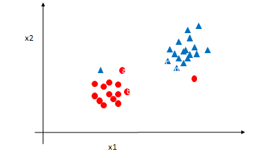
Soft Margin Classification – Noisy data
Noisy data
- What if there is some noise in the data.
- What id the overall data can be classified perfectly except few points.
- How to find the hyperplane when few points are on the wrong side.
### Soft Margin Classification – Noisy data - The non-separable cases can be solved by allowing a slack variable(x) for the point on the wrong side.
- We are allowing some errors while building the classifier
- In SVM optimization problem we are initially adding some error and then finding the hyperplane
- SVM will find the maximum margin classifier allowing some minimum error due to noise.
- Hard Margin -Classifying all data points correctly,
- Soft margin – Allowing some error
### SVM Validation - SVM doesn’t give us the probability, it directly gives us the resultant classes
- Usual methods of validation like sensitivity, specificity, cross validation, ROC and AUC are the validation methods
SVM Advantages & Disadvantages
SVM Advantages
- SVM’s are very good when we have no idea on the data
- Works well with even unstructured and semi structured data like text, Images and trees.
- The kernel trick is real strength of SVM. With an appropriate kernel function, we can solve any complex problem
- Unlike in neural networks, SVM is not solved for local optima.
- It scales relatively well to high dimensional data
- SVM models have generalization in practice, the risk of overfitting is less in SVM.
SVM Disadvantages
- Choosing a “good” kernel function is not easy.
- Long training time for large datasets
- Difficult to understand and interpret the final model, variable weights and individual impact
- Since the final model is not so easy to see, we can not do small calibrations to the model hence its tough to incorporate our business logic.
SVM Application
- Protein Structure Prediction
- Intrusion Detection
- Handwriting Recognition
- Detecting Steganography in digital images
- Breast Cancer Diagnosis
LAB: Digit Recognition using SVM
- Take an image of a handwritten single digit, and determine what that digit is.
- Normalized handwritten digits, automatically scanned from envelopes by the U.S. Postal Service. The original scanned digits are binary and of different sizes and orientations; the images here have been de slanted and size normalized, resultingin 16 x 16 grayscale images (Le Cun et al., 1990).
- The data are in two gzipped files, and each line consists of the digitid (0-9) followed by the 256 grayscale values.
- Build an SVM model that can be used as the digit recognizer
- Use the test dataset to validate the true classification power of the model
- What is the final accuracy of the model?

#Importing test and training data

train_data = numpy.loadtxt('datasets/Digit Recognizer/USPS/zip.train.txt')
test_data  = numpy.loadtxt('datasets/Digit Recognizer/USPS/zip.test.txt')

train_data.shape
test_data.shape
for i in range(0,9):
    data_row=train_data[i][1:]
    #pixels = matrix(as.numeric(data_row),16,16,byrow=TRUE)
    pixels = numpy.matrix(data_row)
    pixels=pixels.reshape(16,16)
    plt.figure(figsize=(10,10))
    plt.subplot(3,3,i+1)
    plt.imshow(pixels)


  #Are there any missing values?
sum(sum(pd.isnull(train_data)))
sum(sum(pd.isnull(test_data)))
#The data are in two gzipped files, and each line consists of the digitid (0-9) followed by the 256 grayscale values.
#The first variable is label
train_data1= pd.DataFrame(train_data)
train_data1[0].value_counts()
#Build an SVM model that can be used as the digit recognizer
########SVM Model Building
#Verify the code with small data
X1=train_data[:5000,range(1,257)]
Y1 =train_data[0:5000,0]
import time
start_time = time.time()
numbersvm = svm.SVC(kernel='rbf', C=1).fit(X1,Y1)
print("---Time taken is %s seconds ---" % (time.time() - start_time))
predict6 = numbersvm.predict(X1)
Y1 = pd.DataFrame(Y1)
Y1[0].value_counts()

predict6=pd.DataFrame(predict6)
predict6[0].value_counts()
#Confusion Matrix
conf_mat = confusion_matrix(Y1,predict6)
conf_mat
Accuracy = numbersvm.score(X1,Y1)
Accuracy
#####Model on Full Data
X2=train_data[:,range(1,257)]
Y2 =train_data[:,0]
import time
start_time = time.time()
numbersvm = svm.SVC(kernel='rbf', C=1).fit(X2,Y2)
print("---Time taken is %s seconds ---" % (time.time() - start_time))
#Confusion Matrix
predict7 = numbersvm.predict(X2)
conf_mat = confusion_matrix(Y2,predict7)
conf_mat
print('Accuracy is : ',numbersvm.score(X1,Y1))
###Out of time validation with test data
Ex1 = test_data[:,range(1,257)]
Ey1 = test_data[:,0]
test_predict = numbersvm.predict(Ex1)
conf_mat = confusion_matrix(Ey1,test_predict)
conf_mat
for i in range(0,9):
    data_row=train_data[i][1:]
    #pixels = matrix(as.numeric(data_row),16,16,byrow=TRUE)
    pixels = numpy.matrix(data_row)
    pixels=pixels.reshape(16,16)
    plt.figure(figsize=(10,10))
    plt.subplot(3,3,i+1)
    plt.imshow(pixels)
#Lets see some errors in predictions images.
# Wrong predictions
wrong_pred = numpy.zeros(2007)
cnt=0
for i in range(0,2007):
    if test_predict[i]!=Ey1[i]:
       wrong_pred[cnt]=Ey1[i]
       cnt= cnt+1
cnt
Conclusion
There are many software tools that are available for SVM implementation SVMs are really good for text classification. They also good at finding the best linear separator. The kernel trick makes SVMs non-linear learning algorithms.Choosing an appropriate kernel is the key for good SVM and choosing the right kernel function is not easy. We need to be patient while building SVMs on large datasets. They take a lot of time for training.