Before start our lesson please download the datasets.
Contents
- Introduction
- Data Frames
- Data Importing
- Working with datasets
- Manipulating the datasets
- Creating new variables
- Sorting
- Removing Duplicates
- Merging
- Exporting the datasets into external files
- Conclusion
Introduction
Data handling is most important skill for any data analyst. As a data analyst we spend fair amount of time in handling or manipulating the data. Before jumping to analysis we have to import the data, accurate and validate the data. Sometimes we may have to merge the data from multiple sources and create consolidated data. Sometime just create new variable in the data. These are the basic skills a data scientist should have to handle a dataset before getting into analysis.
Data Frame
Data Frames are table like structures. It means each column contains measurements on one variable and each row contains one case or one observation for each column. Data Frames are actually python dictionaries in their core. When we are working with datasets or dataframes the first thing to be done is importing ” R-Pandas library “. Pandas library is the easiest one to handle datasets in python.
#Example: How to print a dataframe
import pandas as pd
data = {'name': ['Stan', 'Kyle', 'Eric', 'Kenny'], 'age':[9, 9, 11, 12]}
df = pd.DataFrame(data)
df
Observations
Above results indicates that a dictionary called data has been created which contains one key which is name and the value here is given as list of values which would be ‘stan’,’kyle’,’Eric’ and ‘Kenny’. In previous session any list value as a key-value pair was not present but here we can see that we can enter any list as a value also. Here the 4 values has been created in the “name” and the second key which is “age” has 4 values which corresponds to name. By running this code we would be able to run dictionary and if we want to convert this dictionary into dataframe by using Pandas dataframe function. Always remember in the Pandas dataframe function D and F are capital letters.
Data Importing
Most of the datasets will be imported from external source, dataframes won’t be created by ourselves. Any datasets can be imported and Pythons Panda converts this dataset into dataframe.
Data Importing from CSV Files
Suppose we have external CSV file and which is needed to be imported then we need to use pd.read_csv () function. While using this function the address of the file that needs to be imported should be given. While giving the path use Forward Slash (“/”) or two double backward slashes (“”). The windows style of single back slash (“”) will not work.
#Import Superstore Sales Dataset

import pandas as pd
Sales =pd.read_csv("DataSuperstore Sales DataSales_sample.csv")
print(Sales)
Data Importing from Excel file
For importing data from the excel command is pd.read_excel () function. There is a bit difference in using this function that is we just have to give one extra value that is the name of the sheet because excel has many sheets, so it’s important to specify the name of the sheet which we want to import.
# Import World Bank Indicators dataset

import pandas as pd
wb_data = pd.read_excel("DataWorld Bank DataWorld Bank Indicators.xlsx" , "Data by country",index_col=None, na_values=['NA'])
wb_data.head(10)
Observations
From the above result we observed that there is a constraint na_values = [‘NA’]. It means that any missing values in the dataset are considered as “NA”.When we run the above command we will get the results as shown above.
Basic Commands on Datasets
- Is the data imported correctly? Are the variables imported in right format? Did we import all the rows?
- Once the dataset is inside Python, we would like to do some basic checks to get an idea on the dataset.
- Just printing the data is not a good option, always.
- It is a good practice to check the number of rows, columns, quick look at the variable structures, a summary and data snapshot.
Check list after Importing
There are few things that to be done after importing the dataset.

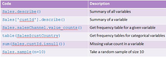
Lab:Basic commands on Datasets
- Import “Superstore Sales DataSales_by_country_v1.csv” data.
- Perform the basic checks on the data.
- How many rows and columns are there in this dataset?
- Print only column names in the dataset.
- Print first 10 observations.
- Print the last 5 observations.
- Get the summary of the dataset.
- Print the structure of the data.
- Describe the field unitsSold, custCountry.
- Create a new dataset by taking first 30 observations from this data.
- Print the resultant dataset.
- Remove(delete) the new dataset.
Subsetting the data
Once the dataset is imported and all the basic operation is performed ,then we might want to create subset of the dataframe and perform analysis on the sub-dataset only. So, how to do the subset of the data? There are many ways to do but we might want our subset to be from any particular rows that we want to select in our new subset or we might want to have a few particular columns in our new subset or we might want a few rows or columns from the previous dataset and create a new subset.
### Import GDP Dataset

import pandas as pd
GDP1=pd.read_csv("DataWorld Bank DataGDP.csv",encoding = "ISO-8859-1")

GDP1.columns.values
Observations
Above results shows the columns that are present in GDP Dataset.
### New dataset with selected rows
gdp=GDP1.head(10)
gdp
Observations
Above results shows first observations of GDP dataset
### New dataset with selected rows based on Index location

gdp1=GDP1.iloc[[2,9,15,25]]
gdp1
### New dataset by keeping selected columns and selected rows

gdp2=GDP1[["Country", "Rank"]][0:10]
gdp2
### New dataset with selected rows and excluding columns
gdp3=GDP1.drop(["Country_code"],axis=1)[0:12]
gdp3
LAB: Sub setting the data
- Data : “./Bank Marketing/bank_market.csv”.
- Create separate datasets for each of the below tasks.
- Select first 1000 rows only.
- Select only four columns “Cust_num” “age” “default” and “balance”.
- Select 20,000 to 40,000 observations along with four variables “Cust_num” “job” “marital” and “education” .
- Select 5000 to 6000 observations drop “poutcome“ and “y”.
Subset with variable filter conditions
Sometimes we want to select a particular variable and we just want to apply condition on that particular variable.
### Import bank_market dataset
bank_data = pd.read_csv("DataBank Tele MarketingBank Tele Marketingbank_market.csv")

### And Condition and Filters
bank_subset1=bank_data[(bank_data['age']>40) &  (bank_data['loan']=="no")]
bank_subset1.head(10)
Observations
Above results indicates the first 10 observations of bank_data subset whose age is greater than 40 and doesn’t have any loan
## OR Condition and Filters
bank_subset2=bank_data[(bank_data['age']>40) |  (bank_data['loan']=="no")]
bank_subset2.head(10)
Observations
Above results shows the first 10 observations of bank_data subset whose age is greater than 40 or who doesn’t have any loan.
### AND, OR condition  Numeric and Character filters

bank_subset3= bank_data[(bank_data['age']>40) &  (bank_data['loan']=="no") | (bank_data['marital']=="single" )]
bank_subset3.head(10)
Observations
Above results shows first 10 observations of bank_data subset whose age is greater than 40 and who doesn’t have any loan or who are not married or staying single.
LAB: Subset with variable filter conditions
Data: “./Automobile Data Set/AutoDataset.csv”
- Create a new dataset for exclusively Toyota cars.
- Create a new dataset for all cars with city.mpg greater than 30 and engine size is less than 120.
- Create a new dataset by taking only sedan cars, keep only four variables(Make, body style, fuel type, price) in the final dataset.
- Create a new dataset by taking Audi, BMW or Porsche company makes. Drop two variables from the resultant dataset(price and normalized losses).
Calculated Fields
Sometimes we want to create a new column based on previous existing columns in our dataset. Let us see how this is done through python code.
### Import AutoMobileDataset

import pandas as pd
auto_data=pd.read_csv("DataAutomobile Data SetAutoDataset.csv")

auto_data['area']=(auto_data[' length'])*(auto_data[' width'])*(auto_data[' height'])

auto_data['area'].head(5)
Observations
Above results shows that a new variable volume has been created with the existing variables “length”, “width” and “height”.
Sorting the data
If you want to sort the dataframe based on any particular column you need to use .sort (). Let us sort Online Retail dataset based on UnitPrice variable.
### Import Online Retail Sales data

Online_Retail= pd.read_csv("DataOnline Retail Sales DataOnline Retail.csv",encoding="ISO-8859-1")

##Sorting Variable UnitPrice in Ascending Order

Online_Retail_sort=Online_Retail.sort_values('UnitPrice')
Online_Retail_sort.head(5)
Observations
Above results shows that a variable UnitPrice have been sorted in ascending order i.e from low values to higher values.
#Sorting variable UnitPrice in Descending Order

Online_Retail_sort=Online_Retail.sort_values('UnitPrice',ascending=False)
Online_Retail_sort.head(5)
Observations
Above results shows that a variable UnitPrice have been sorted in descending order i.e from higher values to lower values.
LAB: Sorting the data
- Import the Auto Dataset.
- Sort the dataset based on length.
- Sort the dataset based on length descending.
Identifying & Removing Duplicates
Duplicates are very big problem when we are going to do some analytics. So, before doing analysis we need to clear duplicates that is present in dataset. To remove duplicates in our dataset we can use the pre-built function pandas ” .duplicated”. Let us see how this works.
## Import Bill Dataset

import pandas as pd
Bill_data=pd.read_csv("DataTelecom Data AnalysisBill.csv")

#Identifying Duplicates

dupes=Bill_data.duplicated()
sum(dupes)
#Dimensions of Bill Dataset

Bill_data.shape
# Removing Duplicates

Bill_data_uniq=Bill_data.drop_duplicates()
Bill_data_uniq.shape
## Identifying duplicates in complaints data based on cust_id

sum(Bill_data.cust_id.duplicated())
#Dimensions of Bill dataset
Bill_data.shape
#Removing Duplicates in cust_id variable

Bill_data_cust_uniq = Bill_data.drop_duplicates(['cust_id'])
Bill_data_cust_uniq.shape
LAB: Handling Duplicates in Python
DataSet: “./Telecom Data Analysis/Complaints.csv”
- Identify overall duplicates in complaints data.
- Create a new dataset by removing overall duplicates in Complaints data.
- Identify duplicates in complaints data based on cust_id.
- Create a new dataset by removing duplicates based on cust_id in Complaints data.
Merging Datasets
In most “real world” situations, the data that we want to use come in multiple sets. We often need to combine these files into a single DataFrame to analyze the complete data. Use pandas pd.merge () function.
What Merge Function will do?
It will take two parameters initially table1 or dataframe1 and 2nd parameter will be table2 or dataframe2 and then third parameter would be on parameter which will have a Key column that we want for merging to be performed on. Most of the times datasets will have a unique columns which we can use as on column or key column then we have a parameter how which allows us what kind of join operation we want to perform. There are four join operations. They are :-
- Left Join.
- Right Join.
- Outer Join .
- Inner Join.
Working of Merging
Merging will combine two tables or dataframes based on a key and return a dataframe. The new dataframe will contain rows based on key column but the entire column will be same.
Working of Joins
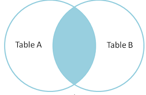
Inner Join
Inner Join combine two dataframes based on a key and will return common rows that have matching values in both the datasets.
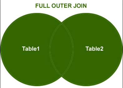
Outer Join
Outer join returns all the rows from both the dataframes based on key but it won’t repeat the common rows i.e, it will take all the columns from both tables but based on key if they are any common rows they won’t be repeated only one of them will be taken into consideration.
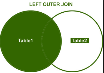
Left Outer Join
Left Join will return all the rows from left table even for the key which doesn’t have value in right table.
Right Outer Join
Right join will return all the rows from right table and even for the key which doesn’t have value in our left table.
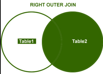
Data sets merging and joining
Here we will import two datasets from Commercial Slot Analysis and we will perform all the four types of joins on the 2 datasets and we will see how it works.
Datasets:
      -TV Commercial Slots Analysis/orders.csv
-TV Commercial Slots Analysis/slots.csv# Import Orders dataset
Orders = pd.read_csv("DataTV Commercial Slots Analysisorders.csv")
#Dimensions of the dataset
Orders.shape
# Import slots dataset
slots = pd.read_csv("DataTV Commercial Slots Analysisslots.csv")

#Dimensions of the dataset
slots.shape
#Identifying duplicates for Unique_id variable in Orders dataset

sum(Orders.Unique_id.duplicated())
#Identifying duplicates for Unique_id variable in Slots dataset

sum(slots.Unique_id.duplicated())
#Removing duplicates for Unique_id variable in Orders dataset

orders1 = Orders.drop_duplicates(['Unique_id'])
sum(orders1.Unique_id.duplicated())
#Removing duplicates for Unique_id variable in Orders dataset

slots1 = slots.drop_duplicates(['Unique_id'])
sum(slots1.Unique_id.duplicated())
#Inner Join

inner_data = pd.merge(orders1, slots1, on = "Unique_id", how = "inner")
inner_data.shape
#Outer Join

Outer_data = pd.merge(orders1, slots1, on = "Unique_id", how = "outer")
Outer_data.shape
#Left Outer Join

Left_outer_data = pd.merge(orders1, slots1, on = "Unique_id", how = "left")
Left_outer_data.shape
#Right Outer Join

Right_outer_data = pd.merge(orders1, slots1, on = "Unique_id", how = "right")
Right_outer_data.shape
LAB: Data Joins
Datasets
     “./Telecom Data Analysis/Bill.csv”
       “./Telecom Data Analysis/Complaints.csv”
- Import the data and remove duplicates based on cust_id.
- Create a dataset for each of these requirements.
- All the customers who appear either in bill data or complaints data .
- All the customers who appear both in bill data and complaints data.
- All the customers from bill data: Customers who have bill data along with their complaints.
- All the customers from complaints data: Customers who have Complaints data along with their bill info.
Exporting the Datasets or dataframe into external file
Once we have created a new dataframe or merged two dataframes we want to create a new data file to save in our hard drive. This can be done by using pandas function .to_csv () to export any data frame into an external .csv file.
Syntax:
dataframe.to_csv (‘path+filename.csv’)
Example:
L_outer_data.to_csv (‘D:Statinferouter_join.csv’)
Conclusion
In this session we started with Data imploring from various sources.
- We saw some basic commands to work with data .
- We also learned manipulating the datasets and creating new variables.
- Sorting the datasets and handling duplicates.
- Joining the datasets is also an important concept.
- There are many more topics to discuss in data handling, these topics in the session are essential for any data scientist .


