Handout – Regression Analysis

You can download the datasets and R code file for this session here.

Regression is one of the most important topics in machine learning. Once we understand the concept of regression, later on understanding remaining models and model building will be much easier. So we need to have a clear understanding of regression before we actually get into a lot of advance topics in machine learning. Let us see the contents.

Correlation
- Correlation between continuous variables
- Correlation between continuous and categorical variables
- Correlation between categorical variables
Regression
- Simple Regression
- R-Squared
- Multiple Regression
- Adj R-Squared
- P-value
- Multicollinearity
- Interaction terms

What is need of correlation?

Is there any association between the hours of study and the grades? Do you think if the hours of study is really high? Can we achieve better grades?
Is there are any association between number of temples or number of churches in a city to that of crime rate? Can you say if there are higher number of temples, then the crime rate is higher or if there are lower number of temples, then crime rate is lower or the opposite is true?
What happens to sweater sales with increase of temperature? Obviously, if the temperature increases people don’t wear sweaters lot then sweater sales might go down. We know there is some association between these two but what exactly is the strength of association?
What happens to the ice-cream sales versus temperature? As the temperature increases ice-cream sales might go up, then what is the strength of association between these two variables?

Correlation Coefficient

Can we compare the association between sweater sales and temperature versus ice-cream sales and temperature? So they are all associations we want to quantify the association. So to quantify the association we use a measure called correlation , so correlation simply quantifies the association, it is a measure of linear association as, if one variable increases what happens to the other variable, does it increase or decrease, correlation quantifies that. So the correlation coefficient ‘r’ is the ratio of variance together, to the of product of separate standard deviations. $Correlation coefficient (r) = \frac{Covariance of XY}{\sqrt(VarianceX* VarianceY)}$ The value of r varies between +1 and -1 (both inclusive).

Correlation 0 | No linear association
Correlation 0 to 0.25 | Negligible positive association
Correlation 0.25-0.5 | Weak positive association
Correlation 0.5-0.75 | Moderate positive association
Correlation >0.75 | Very Strong positive association Same goes for negative correlation as well.
So if the correlation is very close to +1, then we will say there is a higher correlation. If it is more 0.5, then we will say moderate positive association. If it is more than 0.75, then we will say there is very strong positive association. On the other end, if the correlation is less than -0.75, we call it as highly negative, so that is like an inverse relationship, that is, as one increase other one decrease.

So, in the sweater sales example, as the temperature increases, the sweater sales go down, this is an inverse association, which is a negative correlation, where as; in the Ice-cream sales, as the temperature goes up, the ice-cream sales go up as well, so that is a clear positive association. So, to understand correlation we will just do a small exercise, we will take air passenger’s data then we will see what is the correlation between them.

Lab:Correlation Coefficient in R

Let’s do a lab on correlation calculation, we have a dataset called Air Passengers data, then we have to find some correlation in that datasets. We have to find the correlation between number of passengers and promotional budget and also we have to correlation between numbers of passengers and inter metro flight ratio. We can get the dataset inside R. Dim gives us the size of the data. There are 80 rows and 9 columns in this data.

Import Dataset: AirPassengers.csv

air <- read.csv ("R datasetAirPassengersAirPassengers.csv")

We can actually look at the Air Passenger’s data and try to understand what exactly this data contain. It contains week numbers, the number of passengers and the promotional budget that was spent by that particular airline in that particular week. The promotional budget can be the ticket fairs promotions or marketing TV or billboard marketing or everything that is spent on promoting that particular ticket. Do you think if you spent a lot of money on marketing and giving lower price ticket will increase a number of passengers? It looks like intuitively that true number of passengers may be high whenever we increase or decrease, number of passengers will be high if we increase the promotional budget that means a simple way of looking at it is if you are offering your airline tickets at a cheaper fares definitely people will go ahead and buy the tickets.

Find the correlation between number of passengers and promotional budget.

cor(air$Passengers, air$Promotion_Budget)

## [1] 0.965851

So we find the correlation to be 96% which indicates that there is very high positive correlation between number of passengers and promotional budget. We can expect a lot of passengers when we actually spent a lot of money on promoting or on giving a lot of discounts and coupons to the users. Let us plot the relationship between the number of passengers and the promotional budget.

plot(air$Passengers, air$Promotion_Budget)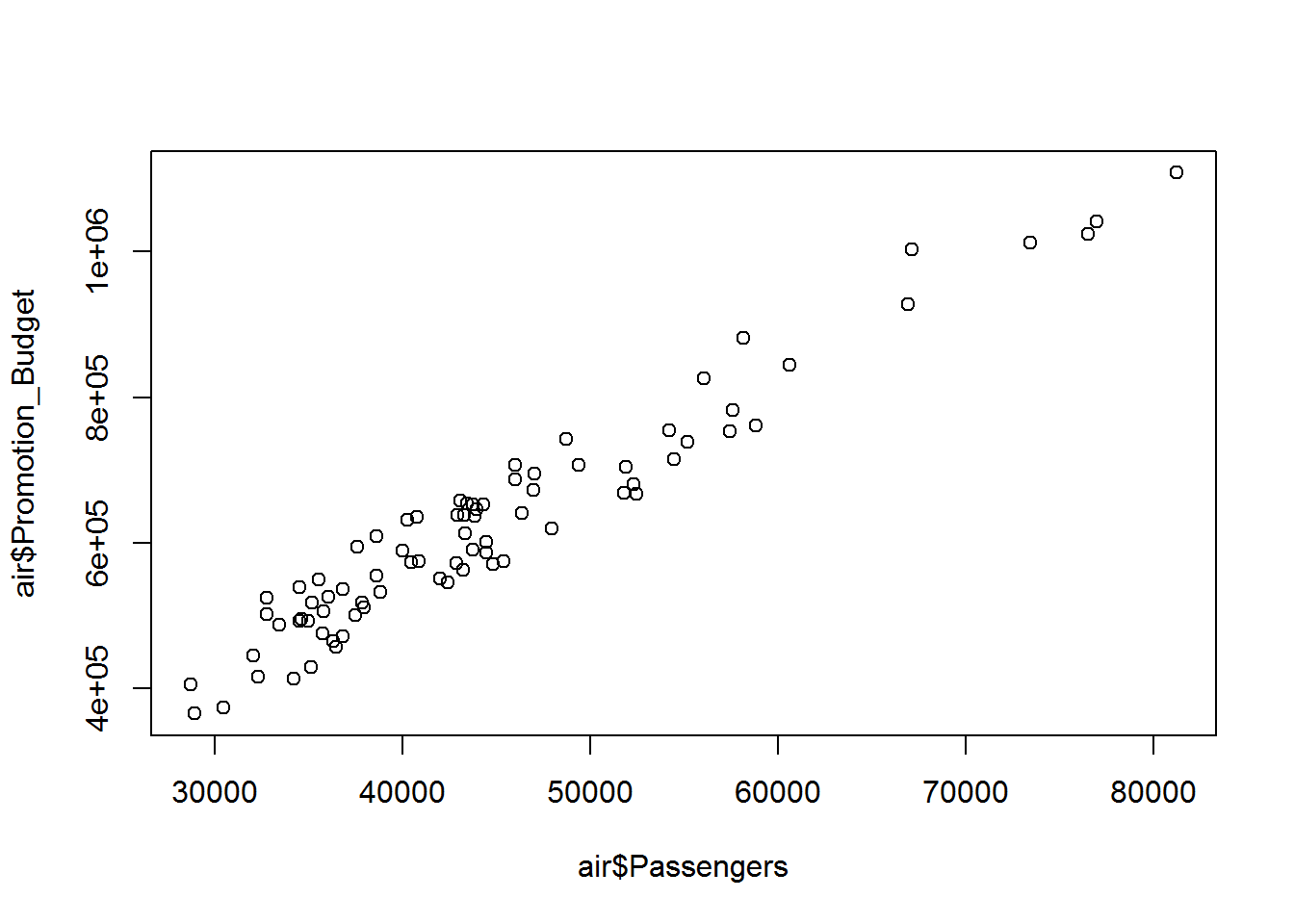

Find the correlation between number of passengers and Service_Quality_Score.

cor(air$Passengers, air$Service_Quality_Score)

## [1] -0.88653

plot(air$Passengers, air$Service_Quality_Score)

Will there be any association between holiday week and number of passengers? Quantify the association between holiday week and passenger count. What is the correlation?

cor(air$Passengers, air$Holiday_week)

## Error in cor(air$Passengers, air$Holiday_week): 'y' must be numeric

Few weeks have delayed flights. Is there any association between passengers and flight cancelation?

cor(air$Passengers, air$Delayed_Cancelled_flight_ind)

## Error in cor(air$Passengers, air$Delayed_Cancelled_flight_ind): 'y' must be numeric

Correlation – Not as easy as you thought

The correlation coefficient that we have calculated in the previous example is called Pearson correlation. It is used to find the correlation between two continuous variables. Pearson correlation coefficient, named after the inventor Pearson works only when both the variables are continuous. For example, in the given dataset of Air passenger one of the variable can be number of passengers and another variable can be promotional budget as both of them are continuous variables, we can use pearson correlation on these variable for finding the correlation between them. What if we are trying to find the correlation between an indicator variable and continuous variable? To know what an indicator variable is; let us look at the Air passenger dataset. Holiday week is an indicator variable as it has only two values Yes or No. There are cases where pearson correlation coefficient does not work. Let us look at those cases. By using Pearson correlation coefficient we can’t find correlation between Holiday week and number of Passengers as one of those variable is indicator and other is continuous. Pearson correlation coefficient fails if we tried to find the correlation between delayed fight indicator and number of passengers because delayed flight indicator is an indicator variable and the number of passengers is a continuous variable. Pearson correlation coefficient fails between two indicator variables such as bad weather and technical issue as none of those variables are a continuous variable.So we need to use some specific correlation coefficient depending upon the type of the data that we are dealing with.

Beyond Pearson Correlation

Depending upon types of the variables we can use relevant correlation coefficient. Pearson ‘r’ correlation coefficient works perfectly when both the variables are continuous. If one of the variable is ordinal/ranked/discrete, and other one is continuous/quantitative then we can use Biserial correlation coefficient. If one of the variable is nominal/categorical, and other one is also nominal/categorical then we can use Phi,Contingency correlation coefficient. There is various kind of correlation coefficient but the most widely used among them is Pearson correlation coefficient. Depending upon the type of the problem we have to choose the correlation coefficient. R has all the packages support for calculating the various kinds of correlation coefficients. You can refer to this table for better understanding about choosing the right correlation measure for the different type of variables. Correlation coefficient measures for different types of data

Variable Y	Quantitative /Continuous X	Ordinal/Ranked/Discrete X	Nominal/Categorical X
Quantitative Y	Pearson r	Biserial (r_b)	Point Biserial (r_{pb})
Ordinal/Ranked/Discrete Y	Biserial (r_b)	Spearman rho/Kendall’s	Rank Biserial (r_{rb})
Nominal/Categorical Y	Point Biserial (r_{pb})	Rank Biserial (r_{rb})	Phi, Contingency Coeff, V

Correlation between Continuous and Categorical-Biserial

It is used to find the correlation between an indicator variable and a continuous variable. Biserial correlation takes one of the levels as reference while calculating the correlation. The equation for biserial can be, $r_{pb} = \frac{M_1 - M_0}{s_n}\sqrt{\frac{n_1n_0}{n^2}}$ whereas, $M_1$ being the mean value on the continuous variable X for all data points in group 1, $M_0$ the mean value on the continuous variable X for all data points in group 2, $n_1$ is the number of data points in group 1, $n_0$ is the number of data points in group 2 and n is the total sample size while $s_n$ is the standard deviation of X. ${S_n} = \sqrt{ \frac{\sum_{i=1}^n (X_i - \bar{X})^2}{n}}$

LAB: Biserial Correlation coefficient

Find the correlation between
- 1. Number of passengers and Holiday week
- 1. Number of passengers and Delayed_Cancelled_flight_ind
Is there any association between Bad_Weather_Ind and Delayed_Cancelled_flight_ind?
Is there any association between technical issues and Delayed_Cancelled_flight_ind. Are the flights getting delayed by technical issues?

Solutions

Find the correlation between
- 1. Number of passengers and Holiday week

library("ltm")

## Warning: package 'ltm' was built under R version 3.3.2

## Loading required package: MASS

## Loading required package: msm

## Warning: package 'msm' was built under R version 3.3.2

## Loading required package: polycor

## Warning: package 'polycor' was built under R version 3.3.2

biserial.cor(air$Passengers, air$Holiday_week)

## [1] -0.8161492

Using ‘1’ as the reference level (High level). Passenger’s count vs. zero to one in Holiday_week :

biserial.cor(air$Passengers, air$Holiday_week, level = 2)

## [1] 0.8161492

Using ‘0’ as the reference level(High level). Passenger’s count vs. one to zero in Holiday_week :

biserial.cor(air$Passengers, air$Holiday_week, level = 1)

## [1] -0.8161492

Find the correlation between
- 1. Number of passengers and Delayed_Cancelled_flight_ind

biserial.cor(air$Passengers, air$Delayed_Cancelled_flight_ind, level = 2)

## [1] 0.1154955

Is there any association between Bad_Weather_Ind and Delayed_Cancelled_flight_ind?

biserial.cor(air$Bad_Weather_Ind, air$Delayed_Cancelled_flight_ind, level = 2)

## Error in biserial.cor(air$Bad_Weather_Ind, air$Delayed_Cancelled_flight_ind, : 'x' must be a numeric variable.

Is there any association between technical issues and Delayed_Cancelled_flight_ind. Are the flights getting delayed by technical issues?

biserial.cor(air$Technical_issues_ind, air$Delayed_Cancelled_flight_ind, level = 2)

## Error in biserial.cor(air$Technical_issues_ind, air$Delayed_Cancelled_flight_ind, : 'x' must be a numeric variable.

Correlation between Categorical Variables-Phi,Contingency

The Biserial Correlation doesn’t work, if both the variables are binary or categorical. We need to use Phi-Coefficient . In fact there are many measures like chi-square, odds ratio, contingency index that will give us an idea on the association or the independence of two categorical variables. We need to prepare a contingency table before calculating these correlations.

	Y=1	Y=0
X=1	$n_{11}$	$n_{10}$	$n_1$
X=0	$n_{01}$	$n_{00}$	$n_0$
	$n_1$	$n_0$

$\phi = \frac{n_{11}n_{00} - n_{10}n_{01}}{\sqrt{n_1n_0n_0n_1}}$ LAB: Correlation between Categorical Variables

Is there any association between Bad_Weather_Ind and Delayed_Cancelled_flight_ind?
Is there any association between technical issues and Delayed_Cancelled_flight_ind. Are the flights getting delayed by technical issues?
Find correlation between holiday week and delayed flight indicator.

Solutions

Is there any association between Bad_Weather_Ind and Delayed_Cancelled_flight_ind?

library(vcd)

## Warning: package 'vcd' was built under R version 3.3.2

## Loading required package: grid

contin_table<-table(air$Bad_Weather_Ind, air$Delayed_Cancelled_flight_ind)
contin_table

##      
##       NO YES
##   NO  37   3
##   YES  2  38

assocstats(contin_table)

##                     X^2 df  P(> X^2)
## Likelihood Ratio 73.662  1 0.000e+00
## Pearson          61.288  1 4.885e-15
## 
## Phi-Coefficient   : 0.875 
## Contingency Coeff.: 0.659 
## Cramer's V        : 0.875

Is there any association between technical issues and Delayed_Cancelled_flight_ind. Are the flights getting delayed by technical issues?

contin_table<-table(air$Technical_issues_ind, air$Delayed_Cancelled_flight_ind)
contin_table

##      
##       NO YES
##   NO  17  25
##   YES 22  16

assocstats(contin_table)

##                     X^2 df P(> X^2)
## Likelihood Ratio 2.4345  1  0.11869
## Pearson          2.4227  1  0.11959
## 
## Phi-Coefficient   : 0.174 
## Contingency Coeff.: 0.171 
## Cramer's V        : 0.174

No, the strength of association between these variables are very low with Phi-coefficient equal to 0.174.

Find correlation between holiday week and delayed flight indicator.

contin_table<-table(air$Holiday_week, air$Delayed_Cancelled_flight_ind)
contin_table

##      
##       NO YES
##   NO  30  31
##   YES  9  10

assocstats(contin_table)

##                       X^2 df P(> X^2)
## Likelihood Ratio 0.019045  1  0.89024
## Pearson          0.019037  1  0.89026
## 
## Phi-Coefficient   : 0.015 
## Contingency Coeff.: 0.015 
## Cramer's V        : 0.015

From Correlation to Regression

In the previous example, promotion budget and number of passengers are highly correlated. Promotional budget refers to the ticket fares if a lot of offers are given on the ticket fares the number of passengers are high, if less offers are given on ticket fares then number of passenger are low. Correlation coefficient between promotional budget and number of passengers are high, so by using this relationship can we estimate number of passengers given the promotion budget? Now correlation is just a measure of association, it can’t be used for prediction. Given two variable X and Y correlation can tell to what extend those two variables are associated. Correlation fails when given one variable and asked to find the estimation of the other variable. Similarly in the Air Passenger dataset given the value of promotional budget correlation can’t predict the estimation of numbers of passengers. For these kinds of problems we need a model, an equation, or a curve fit for the data which is known as regression line. Correlation just measures the degree or strength of association between two variables but can’t predict the estimation of second variable given the value of first variable.

Regression

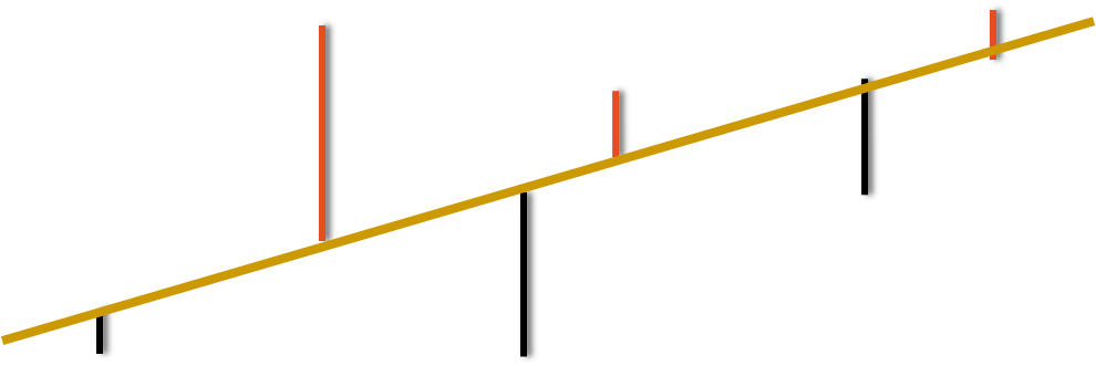
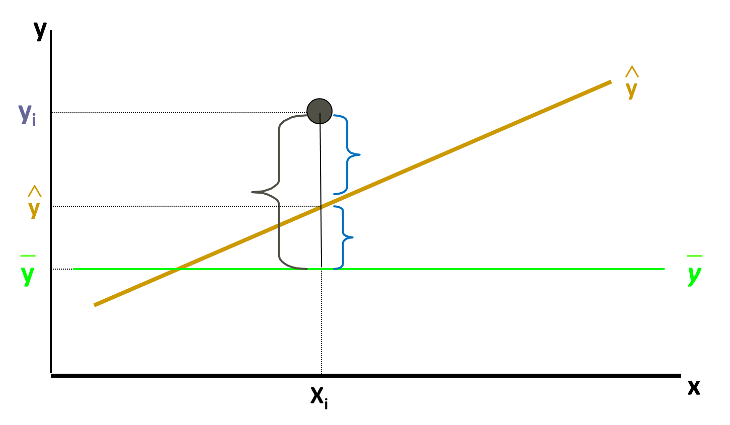
A regression line is a mathematical formula that quantifies the general relation between a two variables one of them are predictor/independent (or known variable x) and the other is target/dependent (or the unknown variable y). In our case promotional budget is the predictor variable that predicts. The number of the passengers are the target variable, this means number of passengers depends upon the promotional budget, promotional budget is independent variable it does not depend on anything. The equation for Regression can be: $y = \beta_0 + \beta_1 x$ Now what is the best fit for given data or what is the best line that goes through the data. The one which goes through the core of the data or the one which minimize the error. Here is the simple example where we can see two variables X and Y and now the question is given the value of X =30, what could be the value of Y?

Regression

Regression Line fitting

In the diagram the blue dots are the data points, now we have to draw the regression line for the given data. On the X and Y axis we have two variables so the regression line equation is $y = \beta_0 + \beta_1$ . In this equation we have to find the value of $\beta_0$ and $\beta_1$ ,by knowing which the imaginary line can be drawn. Regressions line has the minimum error, so this line minimize all the errors but still there are some errors. Such as in the diagram we can see the prediction value of X on the Y is different than the Observed value, so epsilon $\epsilon_i$ is the error at this point, similarly there are multiple error at each points. These error can be divided into the positive errors and negative errors.

Minimizing the Error

So to minimize these errors we need to find the best line, the best fit will have the least error. Some errors are positive and some are negative, therefore taking their sum is not good idea. So the best way is, first we need to square these errors and then find the sum of the square of these errors, and then try to minimize the sum of the square of the error. So we need to find regression line that will minimize the sum of the square of the errors, this is the reason it is called as least square estimation.

Least Squares Estimation

Error can be found by subtracting the actual Y with Y predicted. Y predicted is nothing but $\beta_0 + \beta_1$ whole square. By using the calculus simply we can minimize this function. X: $x_1, x_2, x_3, ... x_n$ Y: $y_1, y_2, y_3, ... y_n$ . Imagine a line through all the points. Deviation from each point is the error or residual. Then we take the square of the deviation. Now our aim is to minimize the sum of squares of deviation. $\sum e^2 = \sum (y - \hat{y})^2$ $\sum e^2= \sum (y - (\beta_0 + \beta_1 x))^2$ The regression coefficient that we would get at the end of the line fitting with the values of $\beta_0 and \beta_1$ would be best possible values which will minimize the sums of squares of error this is called least square estimation. R have a packages which we can use for finding the values of $\beta_0 and \beta_1$ .

LAB: Regression Line Fitting

Import Dataset: AirPassengers.csv
Find the correlation between Promotion_Budget and Passengers
Draw a scatter plot between Promotion_Budget and Passengers. Is there any any pattern between Promotion_Budget and Passengers?
Build a linear regression model on Promotion_Budget and Passengers.
If the Promotion_Budget is 650,000 how many passenger’s can be expected in that week?
Build a regression line to predict the passengers using Inter_metro_flight_ratio

Solution

Import Dataset: AirPassengers/AirPassengers.csv

air <- read.csv ("R datasetAirPassengersAirPassengers.csv")

Find the correlation between Promotion_Budget and Passengers

cor(air$Passengers,air$Promotion_Budget)

## [1] 0.965851

The promotional budget and passengers the correlation is 96% which is a clear indicator of strong relationship.

Draw a scatter plot between Promotion_Budget and Passengers. Is there any any pattern between Promotion_Budget and Passengers?

plot(air$Promotion_Budget,air$Passengers)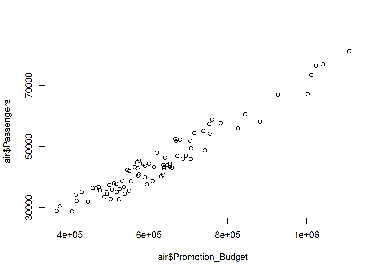

There is a positive pattern between Promotion budget and passengers. We can see there is a very high correlation between these two variables as the promotional budget increase i.e reducing the ticket fares giving the coupons definitely number of passengers are really growing high. If a very less amount is spend on promotional budget in a particular week then the numbers of passengers are low.

Build a linear regression model on Promotion_Budget and Passengers.

For building the regression line we have to use a function called a linear model, lm is the abbreviation for linear model, then use the name of variable whose value needed to be predicted that is the number of passenger in this particular problem, use the symbol ‘~’ tilde then promotion budget which is in the dataset of Air passengers. We need to observe the code, where lm is abbreviation of linear model, Y is the number of passengers and X is the promotional budget.

model1<-lm(air$Passengers~air$Promotion_Budget,data=air)
summary(model1)

## 
## Call:
## lm(formula = air$Passengers ~ air$Promotion_Budget, data = air)
## 
## Residuals:
##     Min      1Q  Median      3Q     Max 
## -5037.6 -2348.6   148.1  2569.3  4851.5 
## 
## Coefficients:
##                       Estimate Std. Error t value Pr(>|t|)    
## (Intercept)          1.260e+03  1.361e+03   0.925    0.358    
## air$Promotion_Budget 6.953e-02  2.112e-03  32.923   <2e-16 ***
## ---
## Signif. codes:  0 '***' 0.001 '**' 0.01 '*' 0.05 '.' 0.1 ' ' 1
## 
## Residual standard error: 2938 on 78 degrees of freedom
## Multiple R-squared:  0.9329, Adjusted R-squared:  0.932 
## F-statistic:  1084 on 1 and 78 DF,  p-value: < 2.2e-16

We can save the output of the above code in the object called model1, so that later we can see the summary of the model. Now we know the values of the [beta_0] and [beta_1 ] [beta_0] is also called as intercept, by using these value of [beta_0] and [beta_1 ] we can find the regression line.

If the Promotion_Budget is 650,000 how many passenger’s can be expected in that week? A new data frame is created for the Promotional budget named as new data. Now using predict function for model1, model1 is the same object which contain the equation $Y = \beta_0 + \beta_1 * X$ where Y=number of passengers and X= promotional budget, with new data.

newdata = data.frame(Promotion_Budget=650000)
predict(model1, newdata)

## Warning: 'newdata' had 1 row but variables found have 80 rows

##        1        2        3        4        5        6        7        8 
## 37231.21 46181.76 45642.49 36475.84 43648.93 34361.58 45478.96 35687.37 
##        9       10       11       12       13       14       15       16 
## 31143.46 43903.97 35520.91 43027.90 33031.89 42010.68 50264.27 38594.96 
##       17       18       19       20       21       22       23       24 
## 52872.05 36040.72 40938.95 58720.33 54174.48 53647.86 36213.01 46722.01 
##       25       26       27       28       29       30       31       32 
## 50399.57 38291.26 37280.85 38762.39 30053.24 46685.99 34089.99 44374.13 
##       33       34       35       36       37       38       39       40 
## 48998.83 37748.09 39502.18 40439.58 45841.07 41012.93 33623.73 42637.56 
##       41       42       43       44       45       46       47       48 
## 48003.02 41228.05 27260.51 26685.22 30209.96 36827.24 35117.92 47059.78 
##       49       50       51       52       53       54       55       56 
## 45152.86 41118.05 42316.33 49552.70 35568.61 55612.21 37843.48 50421.96 
##       57       58       59       60       61       62       63       64 
## 39188.74 39860.40 29482.82 52627.72 47620.47 51007.96 53714.05 71632.69 
##       65       66       67       68       69       70       71       72 
## 70998.02 42249.16 39561.56 46640.24 73695.35 62572.13 48535.48 72489.29 
##       73       74       75       76       77       78       79       80 
## 59982.85 32229.80 47784.98 65762.02 78316.16 45630.81 45524.71 41239.73

Build a regression line to predict the passengers using Inter_metro_flight_ratio

plot(air$Inter_metro_flight_ratio,air$passengers)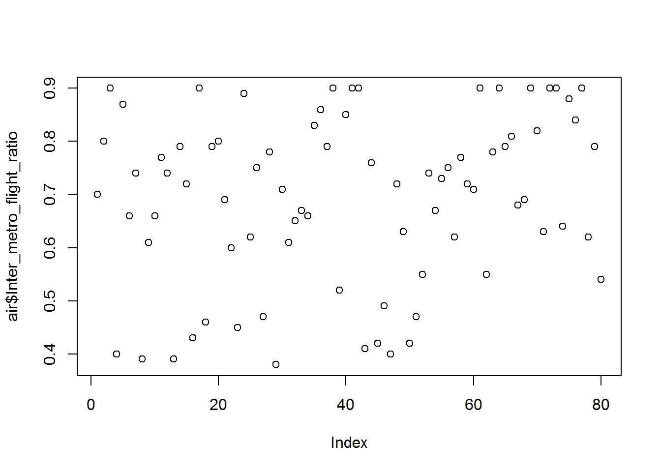

model2<-lm(air$Passengers~air$Inter_metro_flight_ratio,data=air)
summary(model2)

## 
## Call:
## lm(formula = air$Passengers ~ air$Inter_metro_flight_ratio, data = air)
## 
## Residuals:
##    Min     1Q Median     3Q    Max 
## -18199  -6815  -1409   4848  29223 
## 
## Coefficients:
##                              Estimate Std. Error t value Pr(>|t|)    
## (Intercept)                     20441       4994   4.093 0.000103 ***
## air$Inter_metro_flight_ratio    35071       7028   4.990 3.58e-06 ***
## ---
## Signif. codes:  0 '***' 0.001 '**' 0.01 '*' 0.05 '.' 0.1 ' ' 1
## 
## Residual standard error: 9872 on 78 degrees of freedom
## Multiple R-squared:  0.242,  Adjusted R-squared:  0.2323 
## F-statistic:  24.9 on 1 and 78 DF,  p-value: 3.579e-06

How good is my regression line?

What is the proof that the regression line that is built is the best one? What if someone challenges our regression line? What is the accuracy of our model? There is simple way to prove that the regression line that we had drawn is the best one. From the given dataset of Air passengers we can see that if the promotional budget of 517356 is spent then numbers of passengers are 37824. So for checking the accuracy of the regression line that we had drawn, we can re-frame the question as “Predict the number of passengers if the promotional budget is 517356? For the data we already know the answer but still we did the estimation for the numbers of passengers if the Promotional budget spent is of 517356 and the estimation value we got for number of passengers is 37231.21, which is pretty good but yes there are still some errors because the actual value is 37824 and predicted value is 37231.21. When do we say that our regression line is perfect? The regression line is perfect when the estimated value and the predicted value both are exactly same, and the difference or deviation between them is error. Once again to know how well is the regression line that we had drawn, just take a point from the dataset that is already present in the historical data, now just submit the value of the variable X in the regression line then the variable Y’s prediction value will be estimated. If the regression line is the good fit then we can except that Y predicted is the value which is exactly same as the value of Y in the given datasets or we can say Predicted value of Y – Actual value of Y should be zero. If we repeat this for multiple times we can observe that some deviations are positive some are negative this means some time the value of prediction can be higher than the actual value and in some cases the value of prediction can be lower than the actual value. For the best line, Y predicted – Y actual should be zero. So for a good regression line the overall deviations should be less. Since some deviations are positive and some are negative, so we can take sum of square of all such deviations. For a given regression line if the sum of all the square of such deviations is taken in consideration then error should be really less. So while comparing two regression lines look at the sum of the squares of errors of both regression lines, the regression line that makes fewer errors is the better line. $SSE = \sum(y - \hat{y})^2$ IF SSE (sum of squared error) is near to zero then we have a good model. Most of the times standalone SSE is not sufficient. For example if SSE value is 100 so this value is near to 0 or is it far from 0 actually we can’t tell because the value of SSE seems very less if the value of Y is thousands or millions, so the deviation of 100 according to the SSE value is not really high. But if we are working or dealing with fraction or decimals the value of SSE 100 that is really high, so to conclude that if the SSE is having high value or not the variable Y should brought in the picture. So how do we find that how well or correct is our regression line? To answer these just understand the following derivation which will tell us the goodness of fit of our regression line. Error Sum of squares (SSE- Sum of Squares of error) $SSE = \sum(y - \hat{y})^2$ This is sum of squares of errors this should be least for given regression line. Total Variance in Y (SST- Sum of Squares of Total) $SST = \sum(y - \bar{y})^2$ We can rewrite as, $SST = \sum(y - \hat{y} + -\hat{y} - \bar{y})^2$ $SST = \sum(y - \hat{y} + -\hat{y} - \bar{y})^2$ $SST = \sum(y - \hat{y})^2 + \sum(\hat{y} - \bar{y})^2$ $SST = SSE + \sum(\hat{y} - \bar{y})^2$ $SST = SSE + SSR$

Explained and Unexplained Variation

So, total variance in Y is divided into two parts, + Variance that can’t be explained by x (error): SSE + Variance that can be explained by x, using regression : SSR $SST = SSE + SSR$ $Total sum of Squares = Sum of Squares Error + Sum of Squares Regression$ $SST = \sum(y - \bar{y})^2$ $SSE = \sum(y - \hat{y})^2$ $SSR = \sum(\hat{y} - \bar{y})^2$

R-Squared

For a good model SSE should be really low. Another way to look at this would be, the total variance in Y is $SST=SEE + SSR$ , we need to make sure that for really good model. SSE should be minimum, SSR should be maximum, SSE/SST should be always minimum, SSR/SST should always be maximum. The coefficient of determination is the portion of the total variation in the dependent variable that is explained by variation in the independent variable. The coefficient of determination is also called R-squared and is denoted as $R^2$ . $R^2 = \frac{SSR}{SST}$ where 0<= $R^2$ <=1 R squared is the ratio of regression sum of squares to total sum of square; this is also known as explained variance. For a good model explained variance should be near to 100%, the explained variance is 50% then it’s not so good model, this how we can distinguish between a good model and a bad model. For a given model we can look at the value of R squared to tell the given model is good or bad.

Lab: R- Square

So let’s do an lab assignment on R squared model. Previously we have fit the regression line between the numbers of passengers and promotional budget, let’s try to find out the R squared value. So first go to the model object which we have created previously and first run the summary of the model.

What is the R-square value of Passengers vs Promotion_Budget model?
What is the R-square value of Passengers vs Inter_metro_flight_ratio

Solution

What is the R-square value of Passengers vs Promotion_Budget model?

summary(model1)

## 
## Call:
## lm(formula = air$Passengers ~ air$Promotion_Budget, data = air)
## 
## Residuals:
##     Min      1Q  Median      3Q     Max 
## -5037.6 -2348.6   148.1  2569.3  4851.5 
## 
## Coefficients:
##                       Estimate Std. Error t value Pr(>|t|)    
## (Intercept)          1.260e+03  1.361e+03   0.925    0.358    
## air$Promotion_Budget 6.953e-02  2.112e-03  32.923   <2e-16 ***
## ---
## Signif. codes:  0 '***' 0.001 '**' 0.01 '*' 0.05 '.' 0.1 ' ' 1
## 
## Residual standard error: 2938 on 78 degrees of freedom
## Multiple R-squared:  0.9329, Adjusted R-squared:  0.932 
## F-statistic:  1084 on 1 and 78 DF,  p-value: < 2.2e-16

Inside the summary of the model we can find the line that explains the value of R squared. (R^2) is 0.9329

What is the R-square value of Passengers vs Inter_metro_flight_ratio

summary(model2)

## 
## Call:
## lm(formula = air$Passengers ~ air$Inter_metro_flight_ratio, data = air)
## 
## Residuals:
##    Min     1Q Median     3Q    Max 
## -18199  -6815  -1409   4848  29223 
## 
## Coefficients:
##                              Estimate Std. Error t value Pr(>|t|)    
## (Intercept)                     20441       4994   4.093 0.000103 ***
## air$Inter_metro_flight_ratio    35071       7028   4.990 3.58e-06 ***
## ---
## Signif. codes:  0 '***' 0.001 '**' 0.01 '*' 0.05 '.' 0.1 ' ' 1
## 
## Residual standard error: 9872 on 78 degrees of freedom
## Multiple R-squared:  0.242,  Adjusted R-squared:  0.2323 
## F-statistic:  24.9 on 1 and 78 DF,  p-value: 3.579e-06

$R^2$ is 0.242. So let’s now compare this present model with a new model. In this new model we will predict the numbers of passengers using different variable called inter metro flight ratio, if there are more flights between metro cities do you think the number of passengers will depend on that ratio or not. For this we will build a model and check the R squared value for this particular model. The value of R squared is only 25% this means only 25% of the variation can be explained by the inter metro flight ratio. So to predict the number of passenger promotional budget is the better variable.

Multiple Regression

Up till now the regression model we have studied is called as simple regression model.It is called as simple regression model because there is only one predictor variable. In the previous example to predict the number of passengers we were using only one variable that is promotional budget equation; $y = \beta_0 + \beta_1 x$ . where y=number of passengers and x= promotional budget. In real life this is not the scenario just one variable wont impact the overall target; there are multiple variables together which impact the overall target variable, that’s why we need to build multiple regression models. The theory remains same just a small difference is that instead of using one variable x we would be dealing with multiple variables $X_1, X_2$ . And so on. Earlier we were building one regression line in a 2 dimensional plane. But in multiple regression models this would be inclined of plane in 3 dimension system. R squared interpretation will remain same as it was in simple regression

Multiple Regression in R

Build a multiple regression model to predict the number of passengers. So here we will try to predict the number of passengers by using multiple variables such as Promotional budget, inter metro flight ratio, and Service quality score. We are still using the same function lm , for predicting the number of passengers but the only change is that instead of one variables we are using 3 variables to predict from the dataset air

multi_model<-lm(air$Passengers~air$Promotion_Budget+air$Inter_metro_flight_ratio+air$Service_Quality_Score)
summary(multi_model)

## 
## Call:
## lm(formula = air$Passengers ~ air$Promotion_Budget + air$Inter_metro_flight_ratio + 
##     air$Service_Quality_Score)
## 
## Residuals:
##     Min      1Q  Median      3Q     Max 
## -4792.4 -1980.1    15.3  2317.9  4717.5 
## 
## Coefficients:
##                                Estimate Std. Error t value Pr(>|t|)    
## (Intercept)                   1.921e+04  3.543e+03   5.424 6.68e-07 ***
## air$Promotion_Budget          5.550e-02  3.586e-03  15.476  < 2e-16 ***
## air$Inter_metro_flight_ratio -2.003e+03  2.129e+03  -0.941     0.35    
## air$Service_Quality_Score    -2.802e+03  5.304e+02  -5.283 1.17e-06 ***
## ---
## Signif. codes:  0 '***' 0.001 '**' 0.01 '*' 0.05 '.' 0.1 ' ' 1
## 
## Residual standard error: 2533 on 76 degrees of freedom
## Multiple R-squared:  0.9514, Adjusted R-squared:  0.9494 
## F-statistic: 495.6 on 3 and 76 DF,  p-value: < 2.2e-16

The R squared value is around 95% so there is a slight increment in the R squared value by adding these two variables, instead of building model with single independent variable we are using multiple predictor variables for predictions that is called multiple regression model.

Individual Impact of variables

There is no standard rule that if we keep on adding the predictor variables the output mode will be better, this is because in the given dataset sometime we don’t know what variables are impacting the target, and which variables are not impacting the target. In a given regression model suppose we build the output model Y by using 10 predictor variables how will we know that what are the most impacting variables out of those 10 or which variables we can simply drop as it’s effect would be minimum or zero on the output model Y. If a variable is not impacting the model, we can simply drop it, there is no real value in keeping it in the model How do we see the individual impact of the variable? The individual impact of the variables is determined by p value of the t-test. P-value If the p-value is less than 5% then variable has a significant impact, this variable should be kept in the variable.If the p-value is more than 5% then this variable has no impact, we can simply drop this variable as there will be no change in the R squared value. For examples if we are considering the number of laptop sale then there is no point in considering the number of street dogs in the area. By considering the number of street dogs we will not get any help in finding the number of laptop sale so we can simply drop the variable number of street dogs. The p-value can be summarize as , If we drop a low impact variable, there will be no impact on the model, r-square will not change. If we drop a high impact variable, there will be significant impact on the model, r-square will drop significantly. To test: $H_0 : \beta_i = 0$ $H_a : \beta_i \not= 0$ Test Statistic $t=\frac{b_i}{s(b_i)}$ Reject $H_0$ if $t > t(\frac{\alpha}{2};n-k-1)$ or $t > -t(\frac{\alpha}{2};n-k-1)$ In the summary there will be P-value or the probability value. Let’s check the P-value of the variables used in the multi-model in the dataset of Air Passengers. By running the summary of the multi-model which we have already created, we can see the P-value of all the variables those are used. Promotional Budget P-value is less than 5% so this variable is highly impactful. Inter metro flight ratio’s P-value is greater than 5% so we can conclude that this variable is having no impact, keeping or dropping this variable won’t make any changes to output. Service quality score variable is having P-value less than 5% this variable is impactful. By dropping the Inter metro flight ratio variable there would be no impact on the output model. The model can be re-build without using Inter metro flight ratio variable, let’s rename the multi_model as multi_model1 which will have only two variables and they are promotional budget and service quality score. Then by running the summary of multi_model1 value of R squared is almost near the previous model which was having inter metro flight ratio variable, so this conclude that removing the variables whose P-value is greater than 5 won’t affect the model much. By this we can measure the impact of the individual variables and decide based upon their P-value whether these variable should be used or not in building the model. As we already know that promotional budget is highly impactful variable what if we drop the promotional budget variable, will this affect the R squared value? Let’s find out what will happen if we drop a highly impactful variable. This time we will we will drop the variable promotional budget. The r-squared now dropped to 79% from 95%, which proves that the variable is highly impacting. Dropping the variable really impacts model’s overall prediction power. So, if we have 20 predictor variables you want to know which variable is impacting and which variable is not impacting , this can be decided by looking at the P-value.

Adjusted R-Squared

In the regression output summary, you might have already observed the adjusted r-squared field. It is good to have as many as many variables in the data but it’s not recommended to keep on increasing the numbers of variables while building the model , in the hope that R-squared value will also be increasing simultaneously . In fact the R – squared value will never decrease if we keep on adding the variables it slightly increases or it stays same. For example if we build a model using 10 variables with R-squared value is 80% if more 10 variable are added the value of R-squared will never go below 80% either it will stay at 80 or increase slightly. Suppose some the junk variables are added in those extra 10 variables then also R-squared value won’t go below 80%. This is the small problem with R-squared, suppose we keep on adding the junk variables and at some point of time after adding too much junk variables we attain the R-squared value to be 100% which is wrong. So we need a better or slight adjustment to the R-squared value, the original R-squared formula has some issues this issue can be corrected by doing some adjustment. Adjusted R-squared is derived from the r-squared. This adjusted R-squared take cares that if any new variable is added and its impact is not significant the value of Adjusted R-square will not grow. If the new variable which is added is a junk variable then the value of Adjusted R-squared might decrease. So Adjusted R-squared imposes a penalty on adding a new predictor variable, Adjusted R-squared only increases only if the new predictor variables have some significant effect.Adjusted R-squared take care of variable impact as well , if the variable have no impact then, Adjusted R-square won’t increase; if we keep on adding too many variables which are not impactful then the value of Adjusted-r-squared might decrease. $\bar{R}^2 = R^2 - \frac{k-1}{n-k}(1-R^2)$ where n – number of observations and k – number of parameters.

R-Squared vs Adjusted R-Squared

To understand the concept of adjusted R square, we will use an example. Build a model to predict y using x1, x2 and x3. Note down R-Square and Adj R-Square values. Build a model to predict y using x1, x2, x3, x4, x5 and x6. Note down R-Square and Adj R-Square values. Build a model to predict y using x1, x2, x3, x4, x5, x6, x7 and x8. Note down R-Square and Adj R-Square values. Load the dataset into the R by using the R commands. Then build the model 1 named as m1.

Output m1

## 
## Call:
## lm(formula = Y ~ x1 + x2 + x3)
## 
## Residuals:
##      Min       1Q   Median       3Q      Max 
## -1.24893 -0.36289 -0.01435  0.52024  0.73439 
## 
## Coefficients:
##              Estimate Std. Error t value Pr(>|t|)  
## (Intercept) -2.879811   1.162727  -2.477   0.0383 *
## x1          -0.489378   0.369691  -1.324   0.2222  
## x2           0.002854   0.001104   2.586   0.0323 *
## x3           0.457233   0.176230   2.595   0.0319 *
## ---
## Signif. codes:  0 '***' 0.001 '**' 0.01 '*' 0.05 '.' 0.1 ' ' 1
## 
## Residual standard error: 0.7068 on 8 degrees of freedom
## Multiple R-squared:  0.6845, Adjusted R-squared:  0.5662 
## F-statistic: 5.785 on 3 and 8 DF,  p-value: 0.02107

If we look at summary m1 model m1 has an R square of 68% and adjusted R square of 56%. So look at the model m1’s predictor variable’s p-value, there are 3 variables out of which one 1 is non-impactful that’s the variable x1 and remaining two are slightly impactful.

Output m2

## The following objects are masked from adj_sample (pos = 3):
## 
##     x1, x2, x3, x4, x5, x6, x7, x8, Y

## 
## Call:
## lm(formula = Y ~ x1 + x2 + x3 + x4 + x5 + x6)
## 
## Residuals:
##        1        2        3        4        5        6        7        8 
##  0.25902  0.06800  0.45286  0.62004 -1.13449 -0.53961 -0.41898  0.52544 
##        9       10       11       12 
## -0.36028 -0.04814  0.83404 -0.25789 
## 
## Coefficients:
##              Estimate Std. Error t value Pr(>|t|)  
## (Intercept) -5.375099   4.686803  -1.147   0.3033  
## x1          -0.669681   0.536981  -1.247   0.2676  
## x2           0.002969   0.001518   1.956   0.1079  
## x3           0.506261   0.248695   2.036   0.0974 .
## x4           0.037611   0.083834   0.449   0.6725  
## x5           0.043624   0.168830   0.258   0.8064  
## x6           0.051554   0.087708   0.588   0.5822  
## ---
## Signif. codes:  0 '***' 0.001 '**' 0.01 '*' 0.05 '.' 0.1 ' ' 1
## 
## Residual standard error: 0.8468 on 5 degrees of freedom
## Multiple R-squared:  0.7169, Adjusted R-squared:  0.3773 
## F-statistic: 2.111 on 6 and 5 DF,  p-value: 0.2149

In the summary of m2 model the R-squared increased from 68% to 71% whereas Adjusted R-squared dropped from 56% to 37%, this is because in this model m2 there are many non-impactful variables and in the presence of too many non-impactful variable the effect of impact-full variables have gone down resulting in the decreased value of Adjusted -r-squared.

Output m3

## The following objects are masked from adj_sample (pos = 3):
## 
##     x1, x2, x3, x4, x5, x6, x7, x8, Y

## The following objects are masked from adj_sample (pos = 4):
## 
##     x1, x2, x3, x4, x5, x6, x7, x8, Y

## 
## Call:
## lm(formula = Y ~ x1 + x2 + x3 + x4 + x5 + x6 + x7 + x8)
## 
## Residuals:
##       1       2       3       4       5       6       7       8       9 
##  0.4989  0.4490 -0.1764  0.3267 -0.8213 -0.6679 -0.2299  0.2323 -0.2973 
##      10      11      12 
##  0.3333  0.6184 -0.2658 
## 
## Coefficients:
##               Estimate Std. Error t value Pr(>|t|)
## (Intercept) 17.0439629 19.9031715   0.856    0.455
## x1          -0.0955943  0.7614799  -0.126    0.908
## x2           0.0007376  0.0025362   0.291    0.790
## x3           0.5157015  0.3062833   1.684    0.191
## x4           0.0578632  0.1033356   0.560    0.615
## x5           0.0858136  0.1914803   0.448    0.684
## x6          -0.1746565  0.2197152  -0.795    0.485
## x7          -0.0323678  0.1530067  -0.212    0.846
## x8          -0.2321183  0.2065655  -1.124    0.343
## 
## Residual standard error: 0.9071 on 3 degrees of freedom
## Multiple R-squared:  0.8051, Adjusted R-squared:  0.2855 
## F-statistic: 1.549 on 8 and 3 DF,  p-value: 0.3927

In the summary of m3 model the R-squared increased from 71% to 80% whereas Adjusted R-squared dropped from 37% to 28%, this happens only when you are trying to add more predicting variables which are not even related to the target variable.

R-Squared vs Adjusted R-Squared

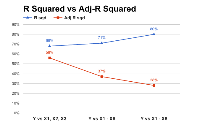
If the values of R-squared and Adjusted-R-squared are nearby this means that there is no junk variables in the data. That means all the variables are impactful or the entire predicting variables that we are considering for building the model from, is impacting target variable in a significant way. If the difference is too high between the values of r squared and adjusted r squared then we can conclude it as there are some variables in the data which are not useful for this particular model.

LAB: Multiple Regression- issues

There are some other issue in multiple regression for understanding these issue lets solve some examples. So let’s do a lab to understand other issue in building the multiple regression line. We will try to understand the problem using an example. There is final exam score data in the dataset import the final exam score data. We need to build a model that predict the final score using the rest of the variables

Import Final Exam Score data
Build a model to predict final score using the rest of the variables.
How are Sem2_Math & Final score related? As Sem2_Math score increases, what happens to Final score?
Remove “Sem1_Math” variable from the model and rebuild the model
Is there any change in R square or Adj R square
How are Sem2_Math & Final score related now? As Sem2_Math score increases, what happens to Final score?
Draw a scatter plot between Sem1_Math & Sem2_Math
Find the correlation between Sem1_Math & Sem2_Math

Solution

First let us import this final score data into the R.

Import Final Exam Score data

final_exam<-read.csv("R datasetFinal ExamFinal Exam Score.csv")

This is final exam data that has final exam marks, sem2 mathematic, sem1 mathematic, sem2 science, sem1 scienUsing four variables that are sem2 mathematic, sem1 mathematic, sem2 science, sem1 science the idea is to predict the final exam score. Create a model called exam_model, and then check the summary of the same.

Build a model to predict final score using the rest of the variables.

exam_model<-lm(Final_exam_marks~Sem1_Science+Sem2_Science+Sem1_Math+Sem2_Math, data=final_exam)
summary(exam_model)

## 
## Call:
## lm(formula = Final_exam_marks ~ Sem1_Science + Sem2_Science + 
##     Sem1_Math + Sem2_Math, data = final_exam)
## 
## Residuals:
##     Min      1Q  Median      3Q     Max 
## -1.7035 -0.7767 -0.1685  0.5386  3.3360 
## 
## Coefficients:
##              Estimate Std. Error t value Pr(>|t|)    
## (Intercept)  -1.62263    1.99872  -0.812 0.426941    
## Sem1_Science  0.17377    0.06281   2.767 0.012279 *  
## Sem2_Science  0.27853    0.05178   5.379 3.43e-05 ***
## Sem1_Math     0.78902    0.19714   4.002 0.000762 ***
## Sem2_Math    -0.20634    0.19138  -1.078 0.294441    
## ---
## Signif. codes:  0 '***' 0.001 '**' 0.01 '*' 0.05 '.' 0.1 ' ' 1
## 
## Residual standard error: 1.33 on 19 degrees of freedom
## Multiple R-squared:  0.9896, Adjusted R-squared:  0.9874 
## F-statistic: 452.3 on 4 and 19 DF,  p-value: < 2.2e-16

From summary it's clear that  R squared  value is  98% adjusted R squared is also 98% this means all the predicting variables that present in the model are having a good impact factor on the target variable. R-Square value of 98%, indicates that the model is a really good one for prediction

How are Sem2_Math & Final score related? As Sem2_Math score increases, what happens to Final score?

Sem2_Math & Final score related are inversely related. As Sem2_Math score increases Final score decreases. Let’s build a new model on the same data, we will drop sem1 mathematics from the model. Let’s use only 3 variables. The most striking difference is in the coefficient of the variable Sem2 mathematics. 4. Remove “Sem1_Math” variable from the model and rebuild the model

exam_model1<-lm(Final_exam_marks~Sem1_Science+Sem2_Science+Sem2_Math, data=final_exam)
summary(exam_model1)

## 
## Call:
## lm(formula = Final_exam_marks ~ Sem1_Science + Sem2_Science + 
##     Sem2_Math, data = final_exam)
## 
## Residuals:
##     Min      1Q  Median      3Q     Max 
## -2.2356 -1.2817  0.0549  0.8363  4.7041 
## 
## Coefficients:
##              Estimate Std. Error t value Pr(>|t|)    
## (Intercept)  -2.39857    2.63229  -0.911 0.373037    
## Sem1_Science  0.21304    0.08209   2.595 0.017302 *  
## Sem2_Science  0.26859    0.06843   3.925 0.000839 ***
## Sem2_Math     0.53201    0.06737   7.897 1.42e-07 ***
## ---
## Signif. codes:  0 '***' 0.001 '**' 0.01 '*' 0.05 '.' 0.1 ' ' 1
## 
## Residual standard error: 1.76 on 20 degrees of freedom
## Multiple R-squared:  0.9808, Adjusted R-squared:  0.978 
## F-statistic: 341.4 on 3 and 20 DF,  p-value: < 2.2e-16

On the same dataset, this variable shows a negative coefficient earlier, but now it is showing a positive coefficient. The newly built model has good r-square value. Its accuracy hasn’t gone down

Is there any change in R square or Adj R square

Model	(R^2)	(Adj R^2)
exam_model	0.9896	0.9874
exam_model1	0.9808	0.978

Both (R^2) and Adjusted(R^2) changed slightly 6. How are Sem2_Math & Final score related now? As Sem2_Math score increases, what happens to Final score? However Sem2_Math & Final score related are now positively related. As Sem2_Math score increases Final score also increases.

Draw a scatter plot between Sem1_Math & Sem2_Math

plot(final_exam$Sem1_Math,final_exam$Sem2_Math)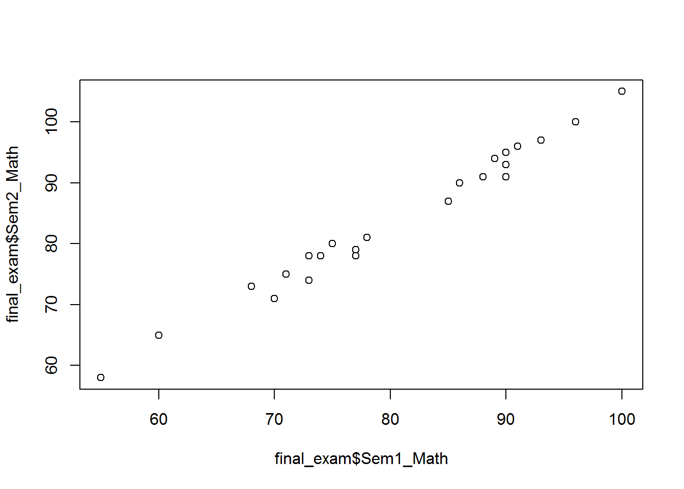

Find the correlation between Sem1_Math & Sem2_Math

cor(final_exam$Sem1_Math,final_exam$Sem2_Math)

## [1] 0.9924948

Multicollinearity

In the above example we found the correlation between the sum1_ math and sem2_maths.we found the correlation value to be 99% between these predictor variables. So now interdependency between these variables is as called multicollinearity. Multicollinearity is an issue because the coefficients that we are getting in the presence of Multicollinearity are not correct because this interdependency really inflates the variance of coefficients, this is a problem. Detection of the Multicollinearity is must and we have to reduce or remove Multicollinearity. In presence of multicollinearity the individual variable impact analysis will lead to wrong conclusions.So we have to first remove or minimize the effect of the Multicollinearity after that only we can trust the coefficient. Multiple regression is wonderful. It allows you to consider the effect of multiple variables simultaneously. Multiple regression is extremely unpleasant because it allows you to consider the effect of multiple variables simultaneously.The relationships between the explanatory variables are the key to understanding multiple regression.

Multicollinearity Detection

$Y = \beta_0 + \beta_1 X_1 + \beta_2 X_2 + \beta_3 X_3 + \beta_4 X_4$

Multicollinearity (or inter correlation) exists when at least some of the predictor variables are correlated among themselves. It might not be just the pairwise correlation. Sometimes many variables together might explain the whole variation in a predictor variable.

Build a model $X_1$ vs $X_2$ $X_3$ $X_4$ find $R^2$ , say $R_1$
Build a model $X_2$ vs $X_1$ $X_3$ $X_4$ find $R^2$ , say $R_2$
Build a model $X_3$ vs $X_1$ $X_2$ $X_4$ find $R^2$ , say $R_3$
Build a model $X_4$ vs $X_1$ $X_2$ $X_3$ find $R^2$ , say $R_4$

Build a regression line $X_1$ vs $X_2$ $X_3$ $X_4$ and find the R Square value, say it $R_1$ . If the $R_1$ value is higher, that is if the $R_1$ value is around 98%, what does this mean ? This means $X_2$ $X_3$ $X_4$ together are explaining 98% of variation in $X_1$ . We can say that $X_1$ is totally dependent on $X_2$ $X_3$ and $X_4$ . $X_1$ is redundant in presence of $X_2$ $X_3$ and $X_4$ . This is a clear indication of multicollinearity. Now if in the second case the $R_1$ value is not really high just around 20% then we can say that $X_1$ is carrying some independent information which is not same as $X_2$ $X_3$ and $X_4$ together. Similarly we can build intermediate models for $X_2$ vs. $X_1$ , $X_3$ , $X_4$ ; $X_3$ vs. $X_1$ , $X_2$ , $X_4$ and $X_4$ vs. $X_1$ , $X_2$ , $X_3$ . With the values of $R_1$ , $R_2$ , $R_3$ and $R_4$ , the respective R-Square values of each of these four models, we can easily detect multicollinearity. Instead of finding these R square we can use another technique called VIF . VIF is derived from the intermediate R-Square value $\frac{1}{(1-R^2)}$ is called VIF. VIF option in SAS automatically calculates VIF values for each of the predictor variables There is a function in R which calculates the VIF value automatically. VIF will be calculated individually for each variable. If a model has 10 independent variables, then we will have 10 VIF values. If a R squared is more than 80% for a particular variable then we can say that Multicollinearity exits. Similarly if we get VIF value more than 5 that mean that the variable can be explained by all the remaining other variables, then this variable can be dropped. Multicollinearity might come in pairs, what do I mean by that is, let us say, in presences of $X_1$ , $X_2$ is redundant, in presence of $X_2$ , $X_1$ is also redundant. So while calculating the VIF of $X_1$ we will use $X_2$ , $X_3$ , $X_4$ then VIF of $X_1$ will be higher. The VIF of $X_2$ will be higher as well because, we are using $X_1$ , $X_3$ , $X_4$ if $X_1$ and $X_2$ are related this does not mean we should drop both $X_1$ and $X_2$ if we drop both then we might lose a whole information together , only one of them should be dropped so that multicollinearity will be lost.

$R^2$	40%	50%	60%	70%	80%	90%
VIF	1.67	2.00	2.50	3.33	4.00	5.00

Multicollinearity Detection in R

Let’s see on the final exam data how to find the VIF values. For calculating the VIF values, we need a package called Car companion to the applied regression. First install the Car package, then build a model named exam.

library(car)
vif(exam_model)

## Sem1_Science Sem2_Science    Sem1_Math    Sem2_Math 
##     7.399845     5.396257    68.788480    68.013104

Now we observe that VIF of all the variables are higher than the 5. But the VIF of Sem1_math and Sem2_Math are really high and we also know that their correlation is also very high. Even though sem1 and sem2 math’s VIF is high, we cannot drop both because, in the presence of Sem2_math , Sem1 is redundant and in presence of Sem1, Sem2 is redundant. Only way to choose the variable which we can drop is the one which is having higher value. So we choose to drop Sem1_Math. Once we drop Sem1_Math, the Sem2_Math gets auto corrected and there will be no Multicollinearity.

vif(exam_model1)

## Sem1_Science Sem2_Science    Sem2_Math 
##     7.219277     5.383840     4.813302

After dropping the Sem1_Math, we get the VIF value of Sem2_math as 4.81 which is less than 5. Observing the VIF value once again, we can see that still there is a Multicollinearity between Sem1_Science and Sem2_Scinece. We will go one step further and drop the Sem1_Science variable and create another model exam_model2.

exam_model2<-lm(Final_exam_marks~Sem2_Science+Sem2_Math, data=final_exam)
summary(exam_model2)

## 
## Call:
## lm(formula = Final_exam_marks ~ Sem2_Science + Sem2_Math, data = final_exam)
## 
## Residuals:
##     Min      1Q  Median      3Q     Max 
## -2.5169 -1.6118 -0.1923  1.4063  3.9476 
## 
## Coefficients:
##              Estimate Std. Error t value Pr(>|t|)    
## (Intercept)  -2.22802    2.96916  -0.750    0.461    
## Sem2_Science  0.37646    0.06134   6.137 4.34e-06 ***
## Sem2_Math     0.62683    0.06386   9.815 2.68e-09 ***
## ---
## Signif. codes:  0 '***' 0.001 '**' 0.01 '*' 0.05 '.' 0.1 ' ' 1
## 
## Residual standard error: 1.986 on 21 degrees of freedom
## Multiple R-squared:  0.9744, Adjusted R-squared:  0.972 
## F-statistic: 399.6 on 2 and 21 DF,  p-value: < 2.2e-16

vif(exam_model2)

## Sem2_Science    Sem2_Math 
##     3.397592     3.397592

By dropping the sem1_Science variable the VIF value is further reduce and the values are less than 5. Now, both the variable’s value is less than 5. So we don’t need to drop any other variables.

Additionally, there is no significant change R-Squared and Adjusted R-Squared values.

Similarly we can do an exercise of finding the Multicollinearity in air passenger data. Identify and eliminate the Multicollinearity in the Air passengers’ model. Dropping of variable should be done one by one we can’t just drop all the variables at once.

Lab: Multiple Regression

Import Dataset: Webpage_Product_Sales/Webpage_Product_Sales.csv
Build a model to predict sales using rest of the variables
Drop the less impacting variables based on p-values.
Is there any multicollinearity?
How many variables are there in the final model?
What is the R-squared of the final model?
Can you improve the model using same data and variables?

Solution

Import Dataset: Webpage_Product_Sales/Webpage_Product_Sales.csv

Webpage_Product_Sales = read.csv("R datasetWebpage_Product_SalesWebpage_Product_Sales.csv")

Build a model to predict sales using rest of the variables

web_sales_model1<-lm(Sales~Web_UI_Score+Server_Down_time_Sec+Holiday+Special_Discount+Clicks_From_Serach_Engine+Online_Ad_Paid_ref_links+Social_Network_Ref_links+Month+Weekday+DayofMonth, data=Webpage_Product_Sales)
summary(web_sales_model1)

## 
## Call:
## lm(formula = Sales ~ Web_UI_Score + Server_Down_time_Sec + Holiday + 
##     Special_Discount + Clicks_From_Serach_Engine + Online_Ad_Paid_ref_links + 
##     Social_Network_Ref_links + Month + Weekday + DayofMonth, 
##     data = Webpage_Product_Sales)
## 
## Residuals:
##      Min       1Q   Median       3Q      Max 
## -14391.9  -2186.2   -191.6   2243.1  15462.1 
## 
## Coefficients:
##                             Estimate Std. Error t value Pr(>|t|)    
## (Intercept)                6545.8922  1286.2404   5.089 4.69e-07 ***
## Web_UI_Score                 -6.2582    11.5453  -0.542  0.58796    
## Server_Down_time_Sec       -134.0441    14.0087  -9.569  < 2e-16 ***
## Holiday                   18768.5954   683.0769  27.477  < 2e-16 ***
## Special_Discount           4718.3978   402.0193  11.737  < 2e-16 ***
## Clicks_From_Serach_Engine    -0.1258     0.9443  -0.133  0.89403    
## Online_Ad_Paid_ref_links      6.1557     1.0022   6.142 1.40e-09 ***
## Social_Network_Ref_links      6.6841     0.4111  16.261  < 2e-16 ***
## Month                       481.0294    41.5079  11.589  < 2e-16 ***
## Weekday                    1355.2153    67.2243  20.160  < 2e-16 ***
## DayofMonth                   47.0579    15.1982   3.096  0.00204 ** 
## ---
## Signif. codes:  0 '***' 0.001 '**' 0.01 '*' 0.05 '.' 0.1 ' ' 1
## 
## Residual standard error: 3480 on 664 degrees of freedom
## Multiple R-squared:  0.818,  Adjusted R-squared:  0.8152 
## F-statistic: 298.4 on 10 and 664 DF,  p-value: < 2.2e-16

Drop the less impacting variables based on p-values.

From the p-value of the output we can see that Clicks_From_Serach_Engine and Web_UI_Score are insignificant hence dropping these two variables

web_sales_model2<-lm(Sales~Server_Down_time_Sec+Holiday+Special_Discount+Online_Ad_Paid_ref_links+Social_Network_Ref_links+Month+Weekday+DayofMonth,data=Webpage_Product_Sales)
summary(web_sales_model2)

## 
## Call:
## lm(formula = Sales ~ Server_Down_time_Sec + Holiday + Special_Discount + 
##     Online_Ad_Paid_ref_links + Social_Network_Ref_links + Month + 
##     Weekday + DayofMonth, data = Webpage_Product_Sales)
## 
## Residuals:
##      Min       1Q   Median       3Q      Max 
## -14305.2  -2154.8   -185.7   2252.3  15383.2 
## 
## Coefficients:
##                            Estimate Std. Error t value Pr(>|t|)    
## (Intercept)               6101.1539   821.2864   7.429 3.37e-13 ***
## Server_Down_time_Sec      -134.0717    13.9722  -9.596  < 2e-16 ***
## Holiday                  18742.7123   678.5281  27.623  < 2e-16 ***
## Special_Discount          4726.1858   399.4915  11.831  < 2e-16 ***
## Online_Ad_Paid_ref_links     6.0357     0.2901  20.802  < 2e-16 ***
## Social_Network_Ref_links     6.6738     0.4091  16.312  < 2e-16 ***
## Month                      479.5231    41.3221  11.605  < 2e-16 ***
## Weekday                   1354.4252    67.1219  20.179  < 2e-16 ***
## DayofMonth                  46.9564    15.1755   3.094  0.00206 ** 
## ---
## Signif. codes:  0 '***' 0.001 '**' 0.01 '*' 0.05 '.' 0.1 ' ' 1
## 
## Residual standard error: 3476 on 666 degrees of freedom
## Multiple R-squared:  0.8179, Adjusted R-squared:  0.8157 
## F-statistic: 373.9 on 8 and 666 DF,  p-value: < 2.2e-16

Is there any multicollinearity?

library(car)
vif(web_sales_model2)

##     Server_Down_time_Sec                  Holiday         Special_Discount 
##                 1.018345                 1.366781                 1.353936 
## Online_Ad_Paid_ref_links Social_Network_Ref_links                    Month 
##                 1.018222                 1.004572                 1.011388 
##                  Weekday               DayofMonth 
##                 1.004399                 1.003881

No. From the above results it can be seen that there is no multicollinearity.

How many variables are there in the final model?

Eight

What is the R-squared of the final model?

0.8179

Can you improve the model using same data and variables?

Interaction Terms

Adding interaction terms might help in improving the prediction accuracy of the model.The addition of interaction terms needs prior knowledge of the dataset and variables.

web_sales_model3<-lm(Sales~Server_Down_time_Sec+Holiday+Special_Discount+Online_Ad_Paid_ref_links+Social_Network_Ref_links+Month+Weekday+DayofMonth+Holiday*Weekday,data=Webpage_Product_Sales)

summary(web_sales_model3)

## 
## Call:
## lm(formula = Sales ~ Server_Down_time_Sec + Holiday + Special_Discount + 
##     Online_Ad_Paid_ref_links + Social_Network_Ref_links + Month + 
##     Weekday + DayofMonth + Holiday * Weekday, data = Webpage_Product_Sales)
## 
## Residuals:
##     Min      1Q  Median      3Q     Max 
## -7486.3 -2073.0  -270.4  2104.2  9146.2 
## 
## Coefficients:
##                           Estimate Std. Error t value Pr(>|t|)    
## (Intercept)              6753.6923   708.7910   9.528  < 2e-16 ***
## Server_Down_time_Sec     -140.4922    12.0438 -11.665  < 2e-16 ***
## Holiday                  2201.8694  1232.3364   1.787 0.074434 .  
## Special_Discount         4749.0044   344.1454  13.799  < 2e-16 ***
## Online_Ad_Paid_ref_links    5.9515     0.2500  23.805  < 2e-16 ***
## Social_Network_Ref_links    7.0657     0.3534  19.994  < 2e-16 ***
## Month                     480.3156    35.5970  13.493  < 2e-16 ***
## Weekday                  1164.8864    59.1435  19.696  < 2e-16 ***
## DayofMonth                 47.0967    13.0729   3.603 0.000339 ***
## Holiday:Weekday          4294.6865   281.6829  15.247  < 2e-16 ***
## ---
## Signif. codes:  0 '***' 0.001 '**' 0.01 '*' 0.05 '.' 0.1 ' ' 1
## 
## Residual standard error: 2994 on 665 degrees of freedom
## Multiple R-squared:  0.865,  Adjusted R-squared:  0.8632 
## F-statistic: 473.6 on 9 and 665 DF,  p-value: < 2.2e-16

Conclusion

In this chapter, we have discussed what is simple regression, what is multiple regression, how to build simple linear regression, multiple linear regression what are the most important metric that one should consider in output of a regression line, what is Multicollinearity how to detect, how to eliminate Multicollinearity, what is R square what is adjusted R square , difference between R square and Adjusted R-squared, how do we see the individual impact of the variables and etc. This is basic regression class once you get a good idea on regression you can explore more in regression by going through the advance topics like adding the polynomial and interaction terms to your regression line , sometimes they work will charm. Adjusted R-squared is a good measure of training/in time sample error. We can’t be sure about the final model performance based on this. We may have to perform cross-validation to get an idea on testing error. About cross-validation we will talk in future lectures in more detail. Outliers can influence the regression line; we need to take care of data sanitization before building the regression line, because at the end of the day these are all mathematical formula if wrong adjustment is done then the wrong result we will get , so data cleaning is very important before getting into regression.

Select Category

Handout – Regression Analysis

You can download the datasets and R code file for this session here.

Regression

Introduction

Contents

What is need of correlation?

Correlation Coefficient

Lab:Correlation Coefficient in R

Correlation – Not as easy as you thought

Beyond Pearson Correlation

Correlation between Continuous and Categorical-Biserial

LAB: Biserial Correlation coefficient

Solutions

Correlation between Categorical Variables-Phi,Contingency

LAB: Correlation between Categorical Variables

Solutions

From Correlation to Regression

Regression

Regression

Regression Line fitting

Minimizing the Error

Least Squares Estimation

LAB: Regression Line Fitting

Solution

How good is my regression line?

Explained and Unexplained Variation

R-Squared

Lab: R- Square

Solution

Multiple Regression

Multiple Regression in R

Individual Impact of variables

Adjusted R-Squared

R-Squared vs Adjusted R-Squared

Output m1

Output m2

Output m3

LAB: Multiple Regression- issues

Solution

Multicollinearity

Multicollinearity Detection

Multicollinearity Detection in R

Lab: Multiple Regression

Solution

Interaction Terms

Conclusion

Attachments1

$\phi = \frac{n_{11}n_{00} - n_{10}n_{01}}{\sqrt{n_1n_0n_0n_1}}$ LAB: Correlation between Categorical Variables