From Correlation to Regression
In previous section, we studied about Beyond Pearson Correlation
In the previous example of Air Passengers, promotion budget and number of passengers are highly correlated. Promotional budget refers to the ticket fares and if a lot of offers are given on the ticket fares, the number of passengers is high, if fewer offers are given on ticket fares than the number of passengers is low. The Correlation coefficient between promotional budget and the number of passengers are high, so by using this relationship, can we estimate the number of passengers given the promotion budget?
Now the correlation is just a measure of association, it can’t be used for prediction.
Given two variable X and Y, correlation can tell us to what extent those two variables are associated. Correlation fails when given one variable and asked to find the estimation of the other variable. Similarly, in the Air Passenger dataset given the value of promotional budget correlation can’t predict the estimation of numbers of passengers. For these kinds of problems, we need a model, an equation, or a curve fit to the data which is known as the regression line.
Correlation just measures the degree or strength of association between two variables but can’t predict the estimation of the second variable given the value of the first variable.
So what is regression?
A regression line is a mathematical formula that quantifies the general relation between two variables, where one of them is a predictor/independent (or known variable x) and the other is the target/dependent (or the unknown variable y). In our case, the promotional budget is the predictor variable that predicts. The number of the passengers are the target variable, this means the number of passengers depends upon the promotional budget, the promotional budget is an independent variable and it does not depend on anything. Here is the regression line if we have X and Y then we can write them as
Why we need to write the regression line equation in this way will be discussed in further sessions. Now, what is the best fit to the given data or what is the best line that goes through the data?
Here is the simple example where we can see two variables X and Y and now the question is given as the value of X =30 what could be the value of Y?
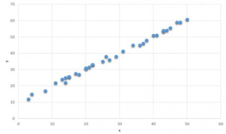
To answer this imagine a straight line that passes through core of the data and we can say that Y=40 when the value of X is 30.

We stared at X=30 and where the value of X and the imaginary lines intersect we can say at that point the value of Y is approx. 40. The imaginary line in the graph which is having least error is called Regression line.The Regression line in the given example formulates the relationship between X and Y where Y is a target variable which depends upon X.
Regression line fitting using least square estimation explains how we fit the line theoretically in the correct way.
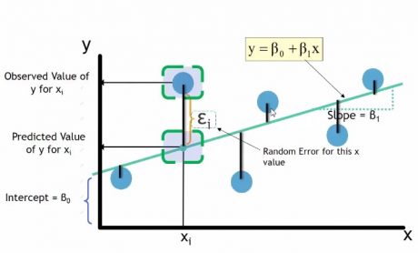
In the diagram, the blue dots are the data points, now we have to draw the regression line for the given data.
On the X axis and Y axis we have two variables, so the regression line equation is , in this equation we have to find the value of
and
,by knowing the value of which the imaginary line can be drawn. Regressions line has the minimum error, so this line minimizes all the errors but still there are some errors. Such as in the diagram we can see the prediction value of X on the Y is different than the observed value, so epsilon is the error at this point, similarly there are multiple errors at each point. These error can be divided into the positive errors and negative errors.

So to minimize these errors we need to find the best line and the best fit will have the least error. Some errors are positive and some are negative. So, taking their sum is not a good idea. The best way is, first we need to square these errors and then find the sum of the square of these errors, and then try to minimize the sum of the square of the errors. We need to find regression line that will minimize the sum of the square of the errors, this is the reason it is called as least square estimation.
For a given X and Y values we will imagine a line through all the points, then we will find the deviation at each points which is called as residual or error, we square up the deviation, in order to find the straight line or regression line by finding the values of the and
in such a way that will minimize the sum of the square of the errors.
Error can be found by subtracting the actual Y with Y predicted. Y predicted is nothing but plus
the whole square. By using the calculus simply we can minimized this function.
The next post is on Practice : Regression Line Fitting in R